
Figures marked "CSIRO", are copyright CSIRO, but please feel free to use them, conditional on the figures not being altered, and their source being acknowledged, and with a link to this site where possible. All other figures are copyright. Please do not copy without the owner's permission.
|
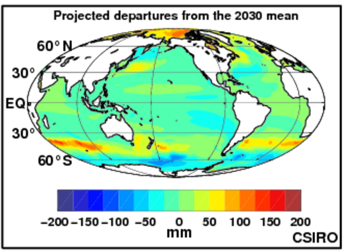
Global projectionsWhen projecting future sea-level rise, we need to recognise that local trends related to decadal variability will be superimposed on the slowly increasing global-mean sea level. However, the long-term climate-change signal will not be uniform, and there will most likely also be a change in the decadal patterns, so providing regional estimates of sea level into the future will be challenging and will require improved understanding of the patterns of 20th century regional changes from observations and models. At this stage there is no agreed pattern for the longer-term regional distribution of projected sea-level rise. There are, however, several features that are common to most model projections - for example a maximum sea-level rise in the Arctic Ocean and a minimum rise in the Southern Ocean south of the Antarctic Circumpolar current. The multi-model mean of the departure of the projected regional sea-level rise from the global-averaged (SRES A1B) projections for 2030 is shown below. (More information about the models used is in the next section.)
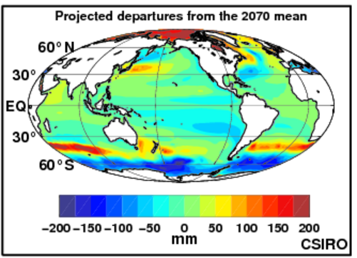
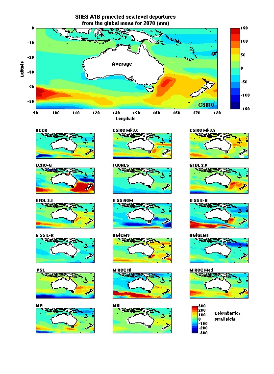
The equivalent for 2070 is:
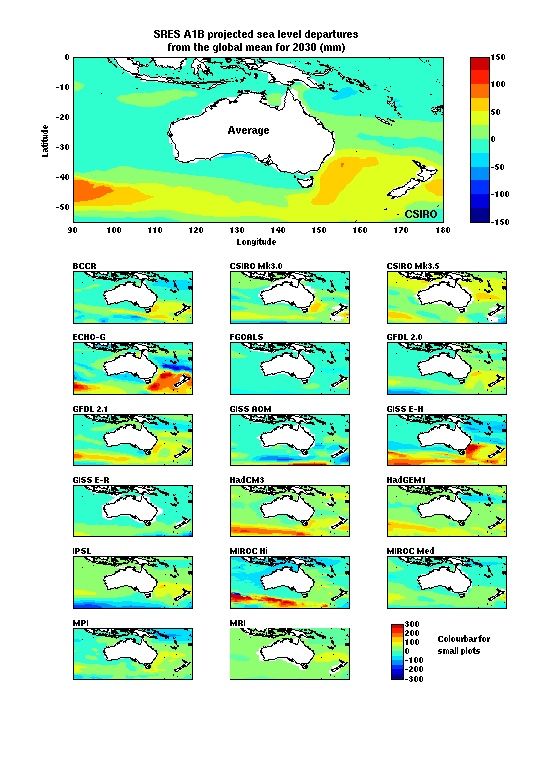
projections for the australian regionIn the Australian region, a common feature in many model projections is a higher than the global average sea-level rise off the south-east coast of Australia and in a band stretching across the Indian and southern Pacific oceans at about 30°-45°S as indicated in the following plots for the A1B SRES Greenhouse Gas Scenario. Regional sea-level projections are currently not available for the A1FI scenario. For both 2030 and 2070, these plots show the departure of the projected regional sea-level rise from the global-averaged projections. Thus to estimate sea-level rise at a particular locations, these distributions need to be added to projections of the global-averaged rise. The results from 17 climate model simulations for the A1B SRES Scenario and the average of these 17 models are shown below. Note that these are results taken directly from the results of the World Climate Research Programme Coupled Model Intercomparison Experiment 3 as used in the IPCC AR4. The models are mostly relatively coarse resolution (1° or greater) although the Miroc Hi model has a resolution of 0.2° x 0.3° Thus the majority of the models do not represent some coastal features well. For more details of the models see the IPCC AR4 report. 2030The figure below shows projected departures from the 2030 global-mean sea level from 17 SRES A1B simulations. The top panel shows the average of all of these simulations, after regridding the results to a common grid, and the smaller panels show the results from the 17 simulations. All panels for the individual model results are presented with the same contour interval (shown by the colourbar at the extreme bottom right) but the average of the models has half the range assigned to the same colour intervals (shown by the colourbar next to this plot). Larger images of each of the individual panels can be obtained by clicking on them (quit the new window to return).
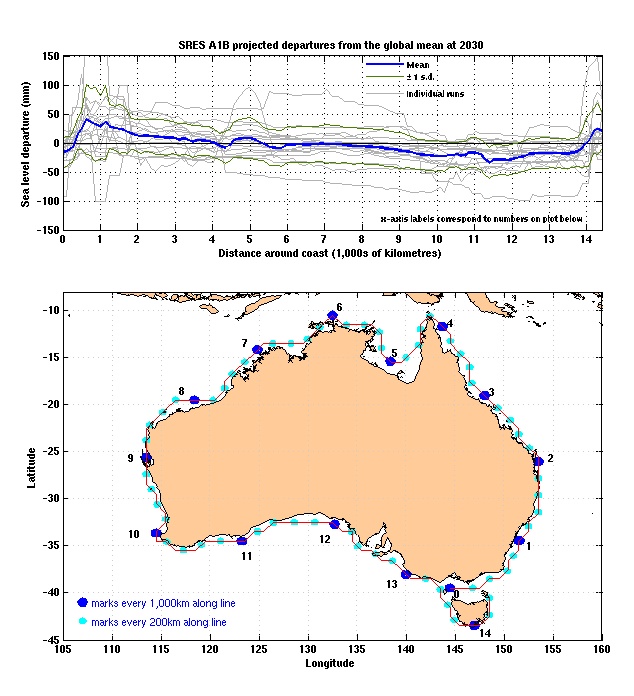
The next figure shows projections around the Australian coastline. To facilitate estimation of projected coastal sea level, the top panel below shows the difference between projected sea level and the global average, plotted around the coastline. The x-axis on the top panel corresponds to distance along the coastline (bottom panel), starting in western Bass Strait, going east, then anti-clockwise around the Australian coast. The top panel shows the average of all models (heavy blue line), the results of the individual models (grey lines) and the model spread (plus- and minus one standard deviation; green line). The bottom panel allows the identification of individual locations adjacent to the coastline. NOTE THAT THESE ARE DEPARTURES FROM THE 2030 GLOBALLY- AVERAGED MEAN PROJECTION FOR THE A1B SRES SCENARIO. The numbers plotted on the top panel (longitude, latitude, distance, mean, standard deviation, minimum and maximum) can be downloaded (.csv file) here. An estimate of regional sea-level rise relative to the land may be obtained by adding the following quantities:
In view of the fact that sea level is presently tracking near the upper bound of the IPCC 2001 projections (see earlier), we expect that global-average sea level may be closer to the upper end of the global projections than the lower end .
2070The figure below shows projected departures from the 2070 global-mean sea level from 17 SRES A1B model simulations. The top panel shows the average of all of these simulations, after regridding the results to a common grid, and the smaller panels show the results from the 17 simulations. All panels for the individual model results are presented with the same contour interval (shown by the colourbar at the extreme bottom right) but the average of the models has half the range assigned to the same colour intervals (shown by the colourbar next to this plot). Larger images of each of the individual panels can be obtained by clicking on them.
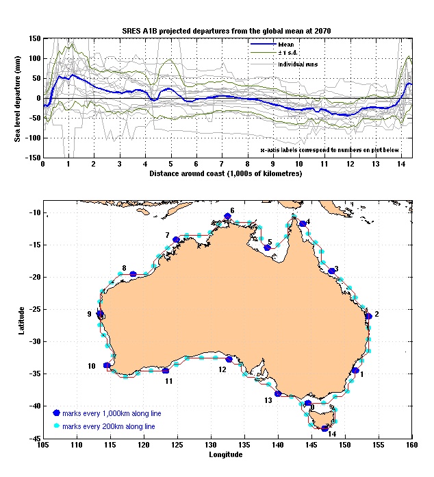
The next figure shows projections around the Australian coastline. To facilitate estimation of projected coastal sea level, the top panel below shows the difference between projected sea level and the global average, plotted around the coastline. The x-axis on the top panel corresponds to distance along the coastline (bottom panel), starting in western Bass Strait, going east, then anti-clockwise around the Australian coast. The top panel shows the average of all models (heavy blue line), the results of the individual models (grey lines) and the model spread (plus- and minus one standard deviation; green line). The bottom panel allows the identification of individual locations adjacent to the coastline. NOTE THAT THESE ARE DEPARTURES FROM THE 2070 GLOBALLY- AVERAGED MEAN PROJECTION FOR THE A1B SRES SCENARIO. The numbers plotted on the top panel (longitude, latitude, distance, mean, standard deviation, minimum and maximum) can be downloaded (.csv file) here. An estimate of regional sea-level rise relative to the land may be obtained by adding the following quantities:
In view of the fact that sea level is presently tracking near the upper bound of the IPCC 2001 projections (see earlier), we expect that global-average sea level may be closer to the upper end of the global projections than the lower end .
In addition to these ocean changes past and ongoing transfers of mass from the ice sheets to the oceans result in changes in the gravitational field and vertical land movements and thus changes in the height of the ocean relative to the land. These large-scale changes, plus local tectonic movements, affect the regional impact of sea-level rise. Withdrawal of groundwater and drainage of susceptible soils can cause significant subsidence. Subsidence of several metres during the 20th century has been observed for a number of coastal megacities. Reduced sediment inputs to deltas are an additional factor which causes loss of land elevation relative to sea level. When using the above projections, care must be taken to allow for these land movements and changes in local wind and atmospheric pressures. AcknowledgementWe acknowledge the modeling groups, the Program for Climate Model Diagnosis and Intercomparison (PCMDI) and the WCRP's Working Group on Coupled Modelling (WGCM) for their roles in making available the WCRP CMIP3 multi-model dataset. Support of this dataset is provided by the Office of Science, U.S. Department of Energy. |
||||
|
Website owner: Benoit Legresy | Last modified 8/08/11
|
![]()
