
Estimating habitat preferences
To determine habitat preferences of SBT involves a number of steps.
- Choose the area of the ocean and timeframe to use for determining habitat preferences. Here we used the GAB (30-40°S, 125-140°E) for months Jan-Mar (corresponding to the main fishing season) in all years for which we have archival tag data, as used in step 4 (1998-2010, 2015-2017).
- Choose the environmental variables to include in the analysis. In our Habitat preference forecasts, we used only sea surface temperature (SST) since this is the only variable currently available from the ACCESS-S seasonal forecast model. However, in our Habitat preference nowcasts, we used both SST and chlorophyll a.
- Extract the environmental data for the entire area and time period chosen.
- Extract the environmental data for only those locations where fish were found within the chosen area and time period. Here we used tracks estimated from SBT with archival tags to determine locations where fish were found within the GAB during Jan-Mar of 1998-2010 and 2015-2017 (all years with data available). Note that the tracks are estimated based on light and temperature data and contain much uncertainty — for more information, see Archival tag tracks.
- Compare the environmental data from the fish locations with the data from the entire area to see which conditions the fish tend to 'prefer'. Because the conditions SBT prefer may depend on their age, we developed separate preference models using locations from fish estimated to be age 2, and from fish estimated to be ages 3-4.
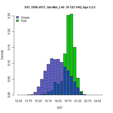
Preferences using SST
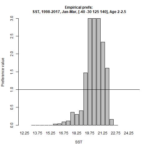
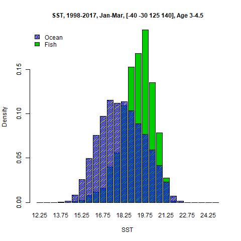
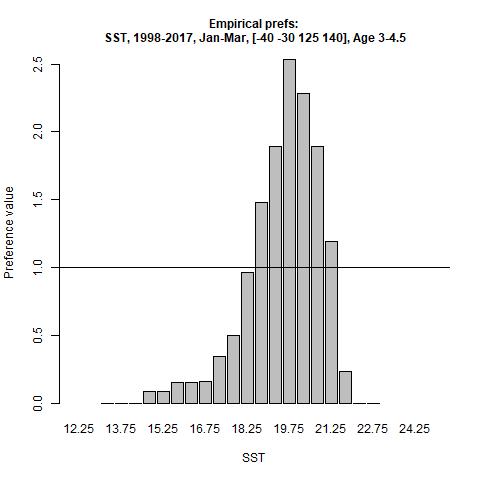
(Left) Distribution of all SST values that occurred in the GAB during Jan-Mar of 1998-2010, 2015-2017 compared with SST values at locations where SBT were found during that same time period. (Right) Preferred SST values, calculated as the ratio of the fish density to the ocean density; preference values greater than 1 indicate SST values where fish density (green bars) is higher than ocean density (blue bars).
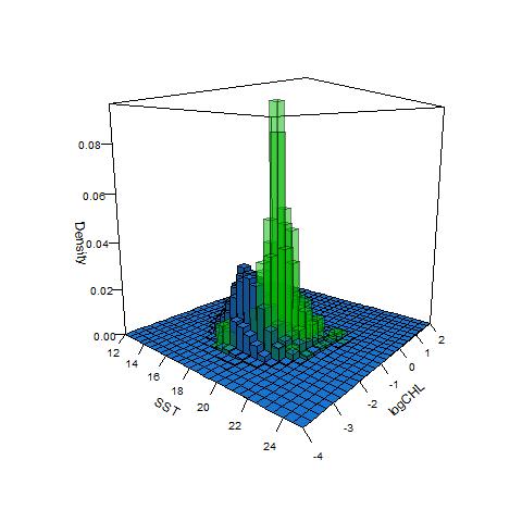
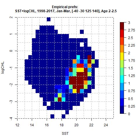
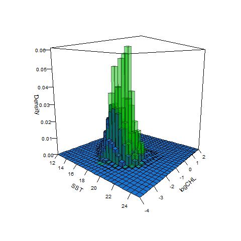
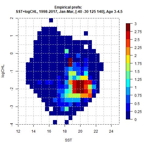
Preferences using SST and chlorophyll a
(Left) Joint distribution of all SST and chlorophyll a (log-transformed, denoted logCHL) values that occurred in the GAB during Jan-Mar of 1998-2010, 2015-2017 compared with SST and logCHL values at locations where SBT were found during that same time period. (Right) Preferred combinations of SST and logCHL, calculated as the ratio of the fish density to the ocean density; preference values greater than 1 indicate combinations of SST and logCHL where fish density (green bars) is higher than ocean density (blue bars).