Methods - habitat preference

The set of predictions of the extent of SBT habitat on the east coast of Australia are based on analyses of current satellite sea surface temperatures (SST), sub-surface temperatures from a CSIRO ocean model incorporating satellite sea surface height data and pop-up tag temperature data for SBT. This model run uses the revised SynTS 3-D ocean product (introduced in 2006) which has improved depth resolution (more layers to a depth of 200 meters: 25 compared with 17). Surface currents are shown on the surface SST map to aid understanding of the ocean dynamics. One habitat preference scenario is now used based on "Percent Habitat Distribution". This is known as Scenario 1: 80%: 15%: 5% (core zone: buffer zone: ok zone)

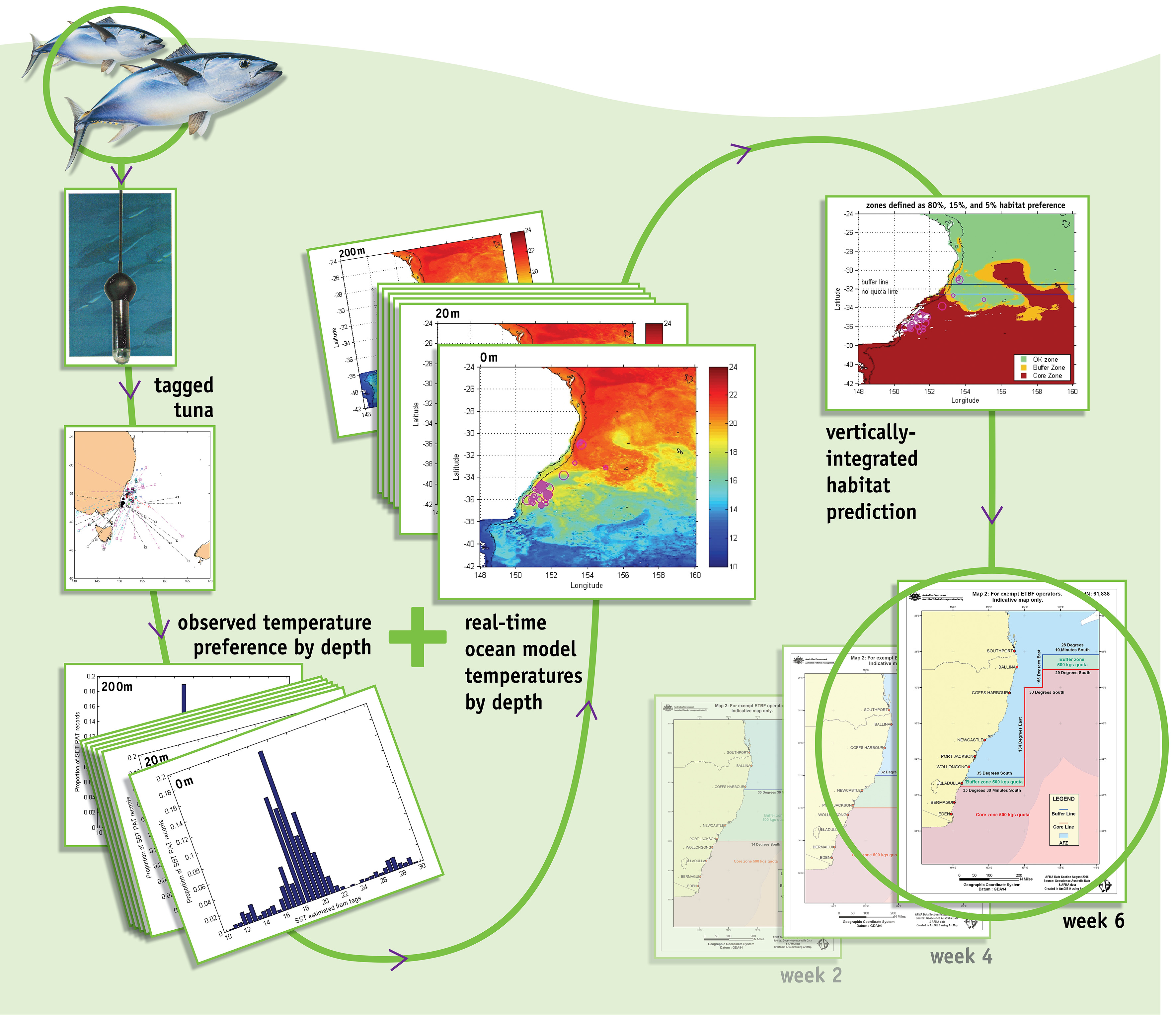
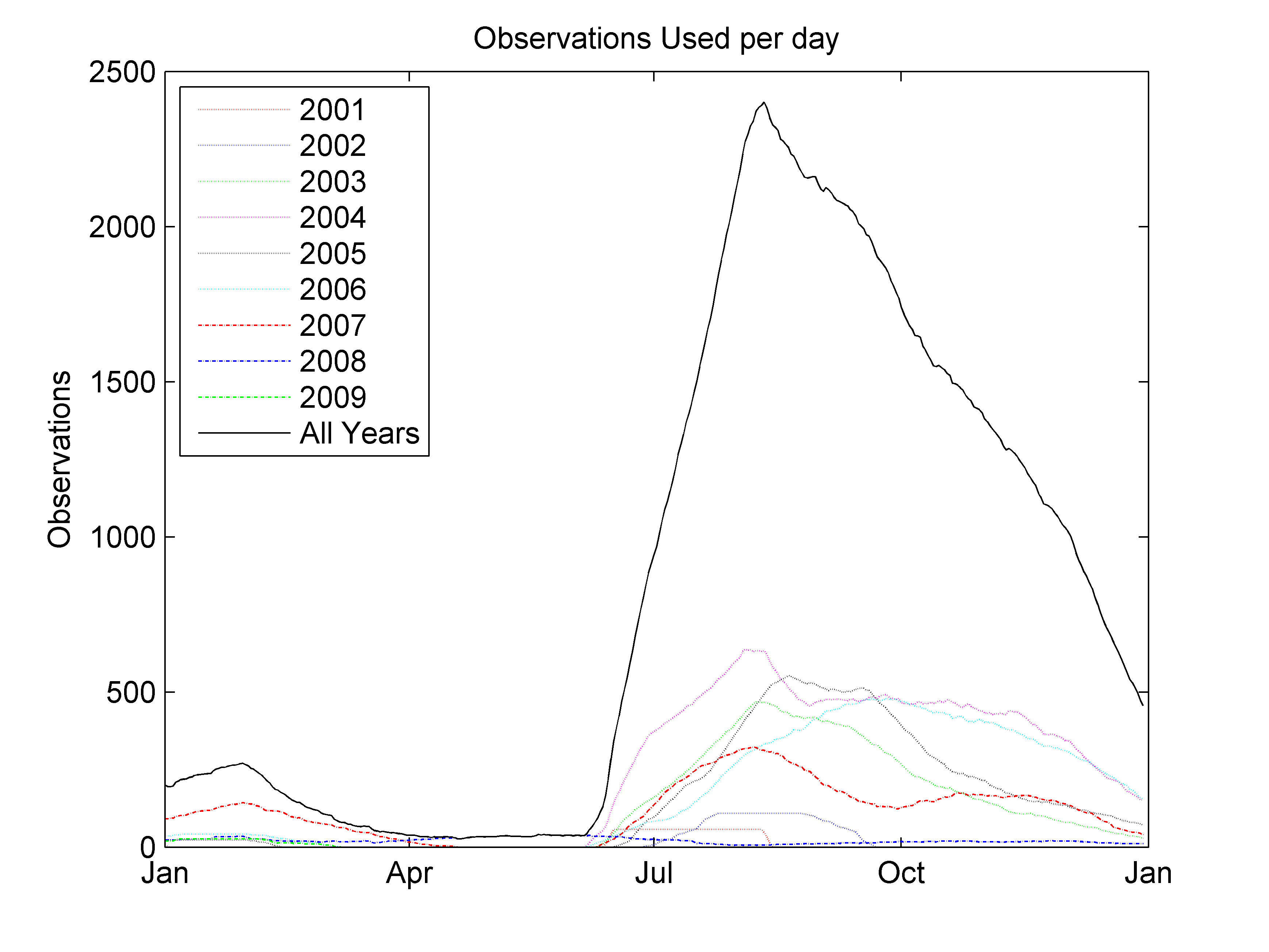
Until the middle of July, tag observations within 70 days of the analysis date will be considered (e.g. May 2 +/- 70 days). This changes to 30 days after that date, as in previous years. The reason for this is that there is limited data in the early part of the year to condition the model. Thus, the current habitat model is conditioned on a pop-up tag dataset consisting of 71 tags for the years 2001-2009 (7656 observations at this time of year). As in 2012, we have included data from SBT tagged in New Zealand, and we acknowledge MFish in New Zealand for the use of these data. Analysis of the data suggests that these animals are suitable to provide additional information on habitat preference in the study area. The pop-up tags provide information about the sub-surface temperatures that the tagged SBT encounters in addition to the SST. This report used SBT sub-surface temperature preferences in combination with a sub-surface temperature oceanographic model to calculate the probability of SBT presence at depths to 200 m. In waters shallower than 200 m the depth integration is only to the maximum depth. These probabilities are then combined over all depths to calculate the probability of SBT presence at a single location.

This same methodology is used to generate the habitat forecast shown here, with the SST and sub surface temperature field being replaced by temperature depth fields obtained from the POAMA model from the Bureau of Meteorology.

The buffer zone climatology compares the average latitudinal position of the buffer zone so far this year with its average position (based on tuna habitat preferences and a 18-year analysis of SST from 1994 to 2013). The climatology is calculated using the subsurface model. Note that the width of the buffer in Figure 4 is due to a persistent inshore filament of buffer water along the coast, and the offshore fraction outside the core of the EAC. This has the effect of moving the most northern 5% of buffer pixels used to calculate the habitat climatology much further north than is apparent in the real-time prediction (e.g. Figure 2). The core zone predictions from the seasonal forecast are shown as red stars on Figure 4. POAMA is not eddy resolving, so there will be dynamic features of the EAC that are not captured in the seasonal forecast. This effect of this is that there are small differences in the core zone prediction (Figure 3a), but overall there is skill in the predictions obtained using POAMA (Hobday et al 2011). The northerly jump in the climatology beginning about April is influenced by limited tag data in this period: the model uses the limited SBT data from the first portion of the year (Figure 5), and then transitions to using the bulk of data available after April. This discontinuity will exist until more data from tags at liberty in February to April are collected.