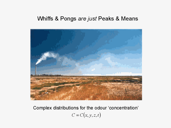
We aim to develop a proper theory for intermittent large concentrations in dispersing atmospheric plumes. Such intermittent behaviour is a necessary component in understanding responses to air-borne odours in the environment, recognising (but for the most part ignoring) the other complex features of odour sensory perception and the multi-species soup of molecules in generic ‘odour’.
Plumes of material in the atmosphere (including malodour) are characterised by concentrations which are complicated functions of space and time. For applications in odour additional sophistication is necessary to predict the fine-scale detail which which can be sensed and elicit responses.
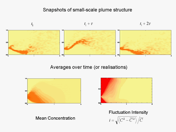
Detailed mathematical model results displayed above in the top panels (obtained using a meandering plume model) show some of the internal structure and detail of plumes at three ordered time instants. Fine scales down to centimetres can be important, which in the atmospheric surface layer plumes means overwhelming information overload for full three dimensional descriptions. Typically average quantities are used to characterise the dispersion, say the mean concentration which is a smooth function on the scale of the surface layer. More detail follows from also knowing the mean-square fluctuations about the mean, also a function of boundary layer scales. However, even these two moments give a limited representation of the full fine-scale variability important in odour problems and more generally we need to know the full probability distribution for concentration, i.e. a detailed mathematical description.
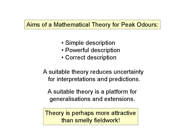
Mathematics gives us an opportunity to represent the necessary detail for the statistics of odour plume variability and make predictions of useful quantities, like peak odour concentrations, odour exposure in finite time, and many more like properties. The generic mathematical characteristics of extreme properties are likely to be as robust as difficult-to-sample field results. Both approaches are needed to make sensible progress. However, despite the need to use sophisticated mathematics for fundamental manipulations, the aim is for simple outcomes relating useful parameters to useful outputs by accurate and easy to use formulae - so called ‘engineering results’.
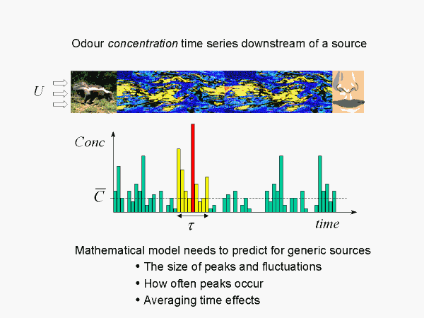
The fine-scale structure of a plume at a sampling point (a nose in the case of odour)is manifest by a sequence of short duration peaks bounded below by zero concentration.In any finite sample there will be a maximum peak and patches of clustered peaks with a net cumulative high odour ‘ concentration’. (Here we necessarily simplify the physiological odour-response intensity to an effective plume concentration). The mathematical model to be constructed must predict properties of the peaks, their clustering, and the effects of sampling. Only the probability distribution of concentrations has enough ‘power’ to include all this information.
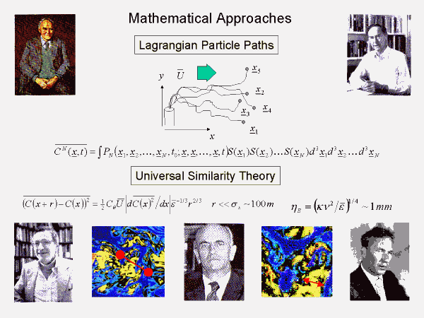
Mathematical approaches to fine scale structure in plumes has a long and productive history. Powerful approaches like Lagrangian particle analysis, similarity theory, dimensional analysis, probability theory, scaling theory and simple mechanics have led to the possibility of immense sophistication in the mathematical representation of plume concentrations. Remarkably many of these ideas can be translated into practical outcomes: for example predicting the probability distribution of concentration in a plume, as functions of robust properties like the mean concentration, the rate of energy dissipation in the plume, the established power law dependence of spatial correlations of concentrations in the plume, mean winds, et cetera.
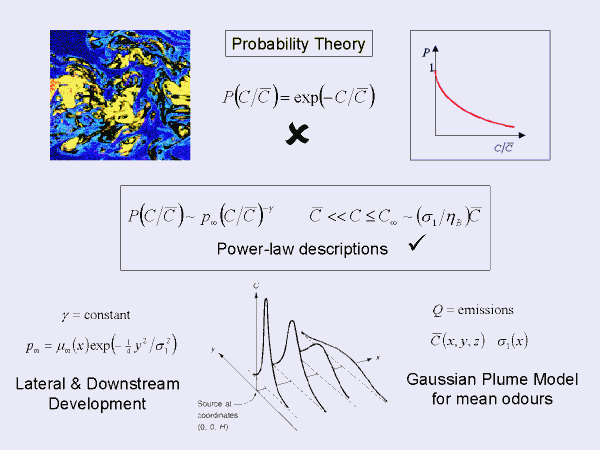
Historically simple functions are arbitrarily selected to ‘best’ model the probability distribution for material in a plume. For example the exponential function is a qualitatively reasonable representation of the proportion of regions exceeding concentration level C (say the yellow or red area in the figure). The proportion of high concentration regions reduces as the level of the concentration threshold is increased (more blue than yellow than red), but the precise fall-off with level is important and is not correctly modelled as exponential decay. Better modelling instead gives a power-law behaviour for the large concentration fall-off. In fact all the details of the power law can be established for generic dispersion problems, predicting the plume-wise development (downstream and lateral) AND MOST CRITICALLY the precise value of the fall-off exponent can be determined.
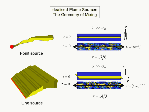
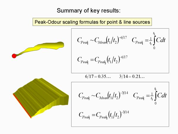
Remarkably the power-law decay exponent is constant in any plume, but it depends on the topology of the plume. A simple continuous point source has the local topology of an instantaneous line source spreading radially (but randomly) in a frame of reference moving with the mean wind. In this view downstream position equates to elapsed time. The exponent derived is the fraction 17/6, that is the fall off is slightly less than inverse third power. The concentration field therefore has a mean and a variance, but higher order moments diverge.
A simple continuous line source on the other hand has the basic topology of an instantaneous plane source spreading normally away from the plane and the exponent derived is the fraction 14/3, that is the fall off is slightly less than inverse fifth power. The concentration field has a mean, variance and skewness but higher-order moments diverge.
More complex behaviour can be described numerically (i.e. multiple sources, sources with finite size). Simple power law behaviour then only occurs strictly in limiting cases, like far from the source so that a point source is appropriate of near to a finite source (say a shed vent) so that locally a line source is appropriate.
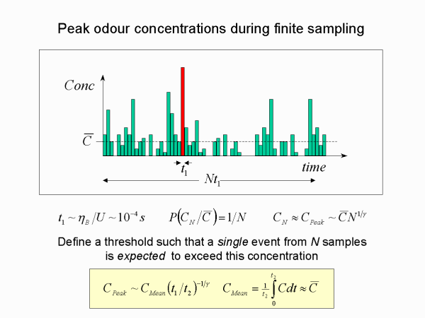
For practical predictions more specific quantities are required, but which ultimately derive from the probability distribution. For example in a sample of N fine-scale concentration peaks, what is the largest peak expected?
We simply define a threshold such that in any given sample of N peaks we expect one peak to have greater than the threshold concentration. For large enough N this simply corresponds to the small probability level of 1/N.
Because the fine-scale peaks have very small effective duration, say milliseconds in the atmosphere, it is possible to attain large N for many practical time samples.
The threshold concentration can easily be determined because of the simple power law tail, immediately giving a formula in terms of ratios of time scales (sample time to fine-scale peak duration time).
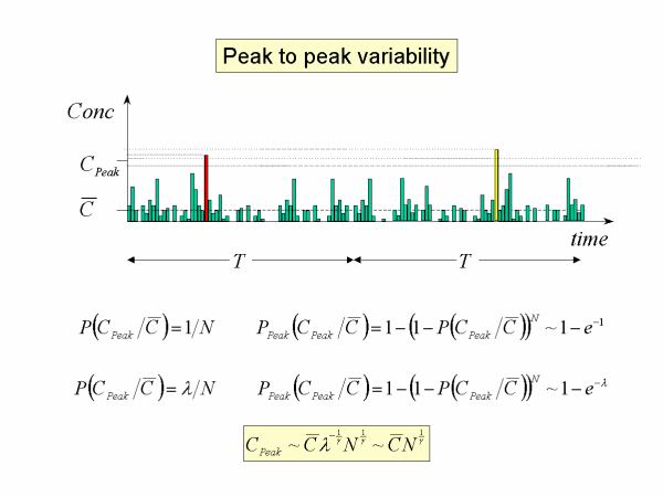
The context of the threshold peak is that distinct samples of duration T will each have an actual peak, sometimes larger sometimes smaller that the threshold defined. In fact, approximately a 0.6 proportion of an ensemble of samples will exceed the threshold. However the mean value of the peaks can be determined precisely to be 1.3 times the threshold, so that by any measure the threshold is a meaningful representation of peak amplitude.
The concept to be aware of here is that the peak amplitude scales according to the formula we are given, that it is a relative measure of peak to mean variability. The absolute measure can be determined by mathematical similarity.
The fine scale peak is interesting but not always the most useful statistic. Instead we are interested in peaks of locally averaged means for short odour response times, say, seconds to minutes. For example, peak one second odours every minute. Now the relative peak odour we have examined is, say, the fine-scale peak in the second-long sample, and the fine scale peak in a minute-long sample. Further it is statistically likely that the largest fine scale peak in a minute corresponds to the largest second-long local average which contains that peak. So by self-similarity we can eliminate the fine-scale variables and relate the minute to second time averaging property or indeed any other time ratio. Self-similarity necessarily gives a precise equality relating the peak to peak variables and is expected to be robust.
Thus mathematical argument leads to generic peak-to-peak power-law predictions that can be readily applied to situations approximated by a continuous point source release (larger exponent so larger peaks for equivalent averaging times) or a continuous line source release. Remarkably, the theoretical estimates are very close to reported observations, bearing in mind the difficulty of sampling for such defined extreme events. (Click here to perform online peak-to-mean concentration calculations.)
The aim of this work is not just to exercise mathematical sophistication but to do so for the purpose of obtaining reliable simple behaviour for quantities of practical interest (namely the prediction of finer scale peaks from readily available average concentrations). Following a rational procedure allows the limitations of such theoretical behaviour to be clearly assessed, and to offer scope for improvement and generalisation. While the outcome has been simple ‘engineering-like’ formulae of greater certainty, which are necessarily the kind of result that finds ready application, it must be remembered that the framework underlying this is essentially conceptually correct, and that manipulations and idealisations within the framework are state-of-the-art. Our predictions are “correct” to best available facts: we may say with certainty that power laws should occur in idealised source releases and that the exponents are universal small-scale properties of turbulent dispersion. Such power laws do give rise to behaviour for clearly defined peak concentrations which agree with observations.