|
|
|
|
|||||||||||||||||||||||||||
|
|
|
|
|||||||||||||||||||||||||||
|
|
Data
Assimilation in a limited-area ocean model Introduction ● Method ● Results link to a
complete list of publications Oke, P. R., and M. Herzfeld,
2009: Ensemble data assimilation in a relocatable ocean model, in preparation. Oke, P. R., G. B.
Brassington, D. A. Griffin and A. Schiller, 2008: The Bluelink Ocean Data
Assimilation System (BODAS), Ocean
Modelling, 21, 46-70,
doi:10.1016/j.ocemod.2007.11.002. Oke, P. R., A. Schiller, G.
A. Griffin, G. B. Brassington 2005: Ensemble data assimilation for an
eddy-resolving ocean model. Quarterly Journal of the Royal Meteorological
Society, 131, 3301-3311. A relocatable ocean atmosphere model (ROAM) has been
developed under the Bluelink project. This system is intended to be used by
both expert and non-expert users, for rapid configuration and execution of
ocean forecasts and hindcasts in any region of the
world’s oceans.
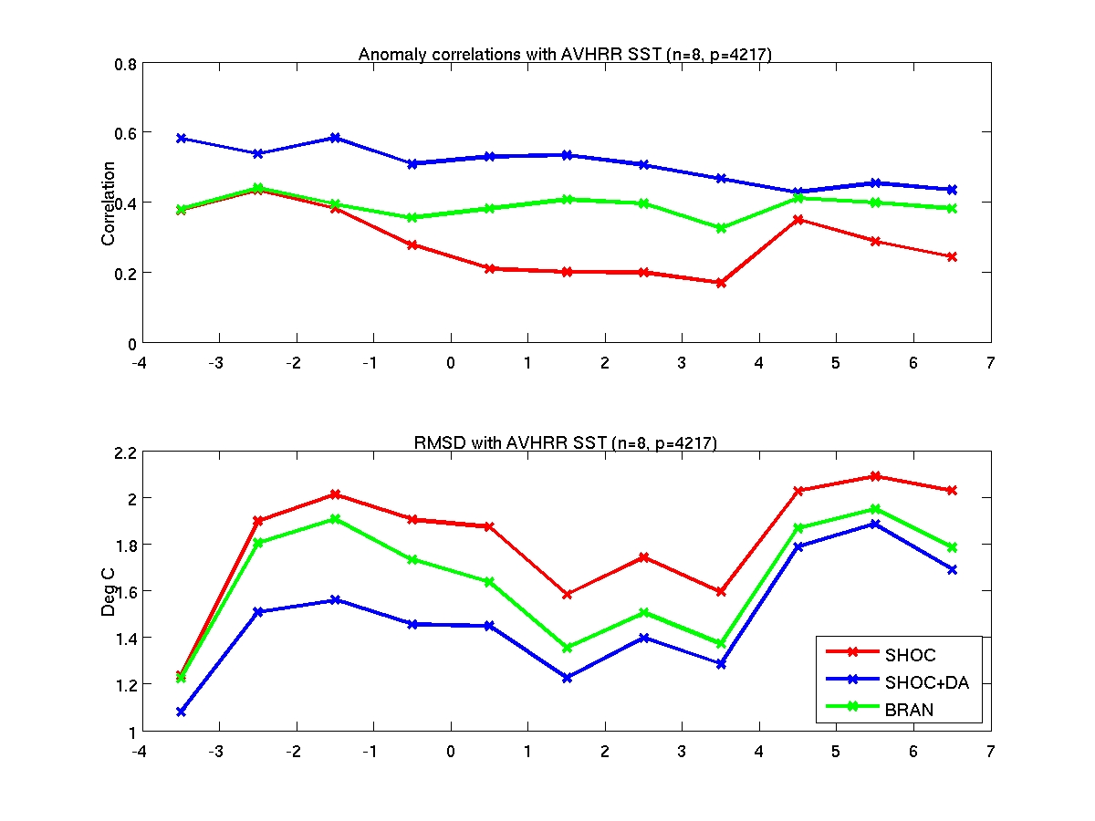
The goal of this study is to improve the performance of the
ocean component of ROAM, in terms of its forecast skill, through data
assimilation.
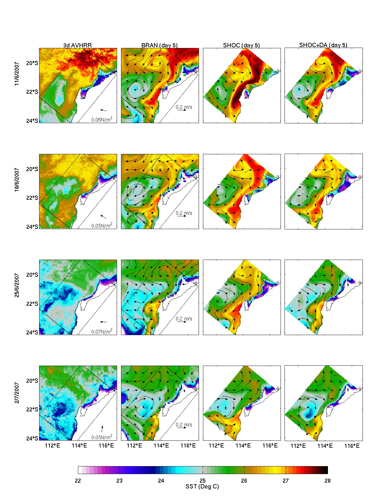
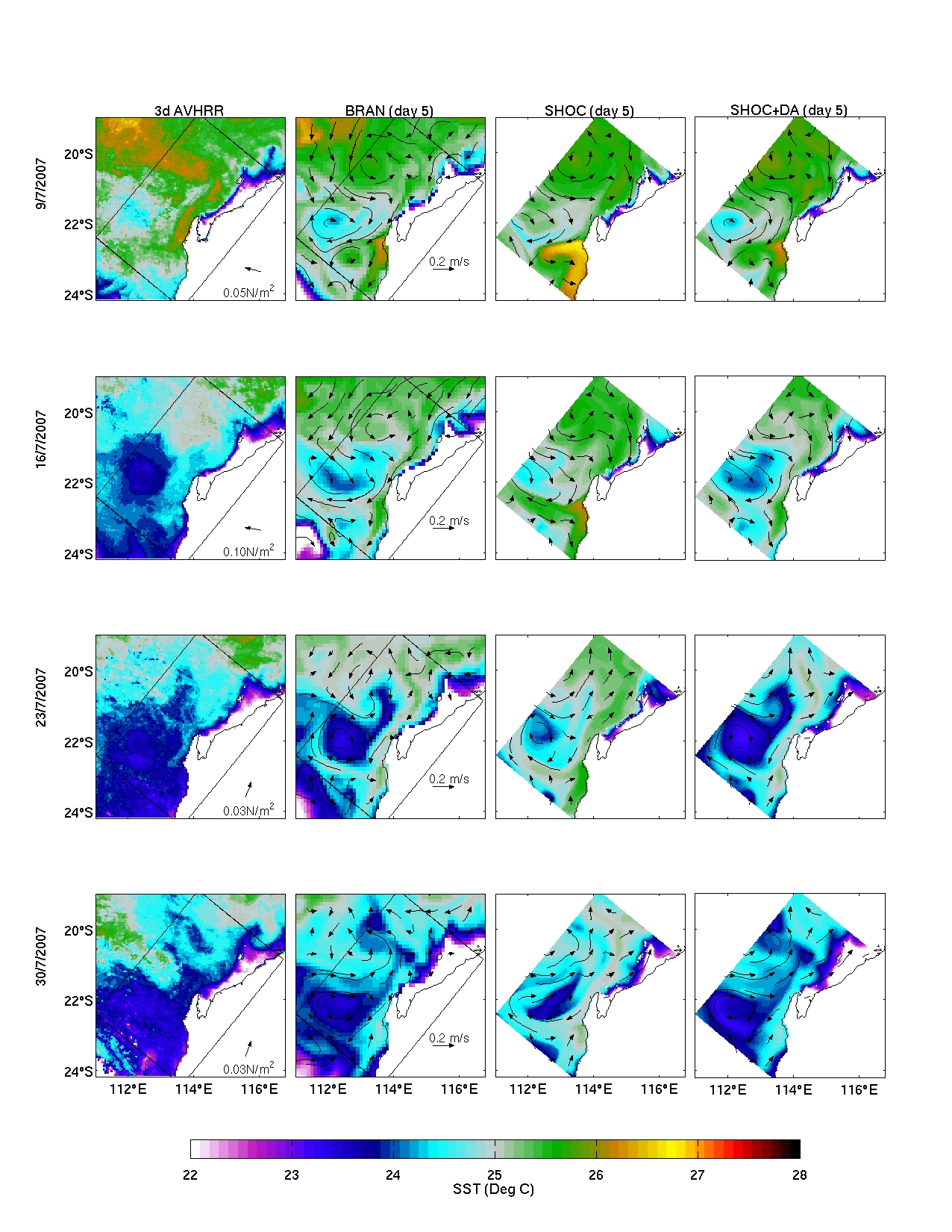
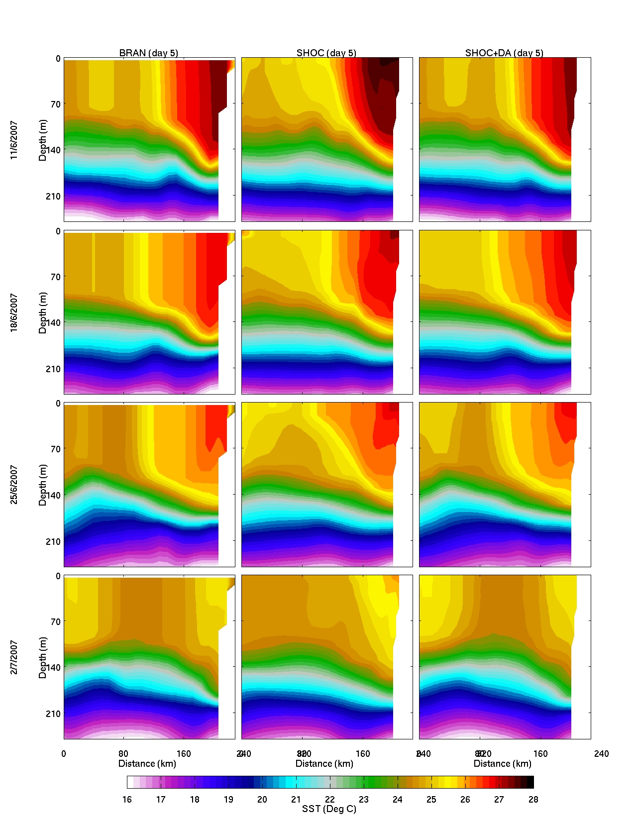
Integration of
a limited-area ocean model (here, SHOC; Herzfeld 2009) usually uses fields a
global eddy-resolving model to prescribe the initial conditions and boundary
fields, for incorporation into the model’s open boundary conditions. An ensemble
data assimilation system (Oke et al. 2008; link) has been developed under the Bluelink project. This system uses a
static ensemble of model anomalies to implicitly represent the background
error covariances used for assimilation. Rather
than constructing, or integrating, a new ensemble for every regional
application, we use the same 1/10 degree resolution global ensemble used by a
global model. We also use fields from the global model as background fields,
and assimilate observations directly into those fields. We then simply use
the new analysis fields, for the region of interest, that represent a combination
of the global model fields and local observations, and initialise and run the
regional model in the usual way. Typically, the
global model has already assimilated the available ocean observations, so
what is to be gained by assimilating again? For computational efficiency, it
is necessary to “super-ob” the observations when assimilating
into the global model. This involves using only a sub-set of the available
observations, and often spatial averaging of the observations prior to
assimilation (yielding “super-obs”).
Because of the limited area, it becomes feasible to improve the global
model’s fields by assimilating more observations, and by assimilating
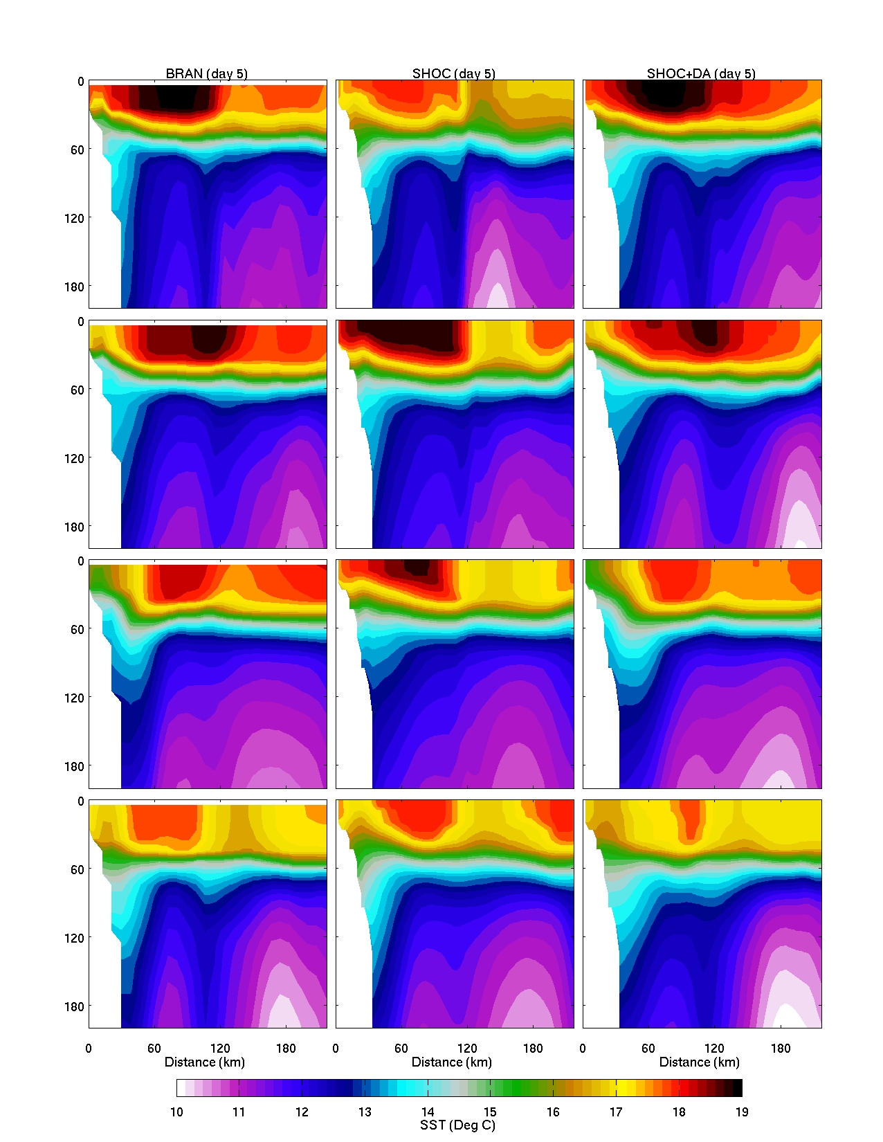
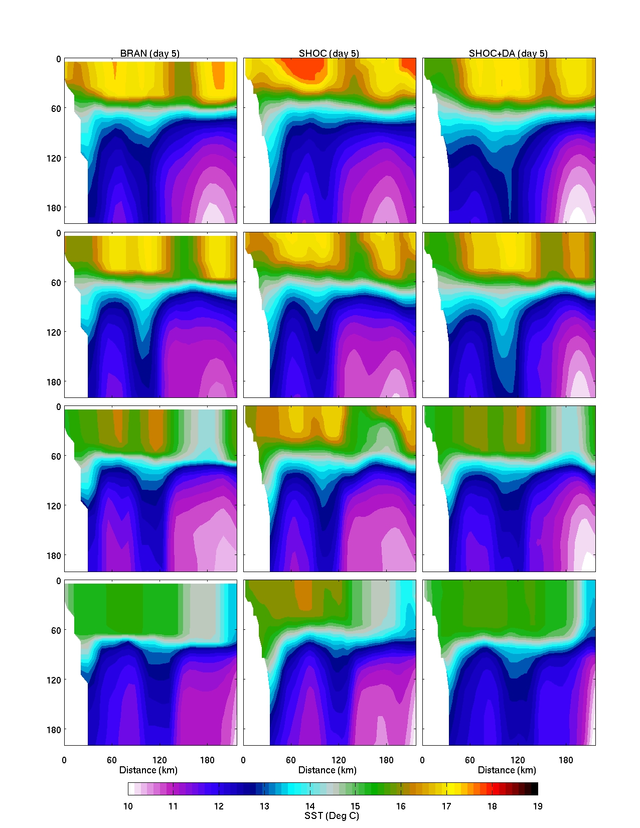
more frequently. Three domains have been considered here. This
includes two regions that are primarily remotely forced, by large-scale
currents, and one region that is strongly locally forced, by winds. These
regions are: -
-
South-Eastern -
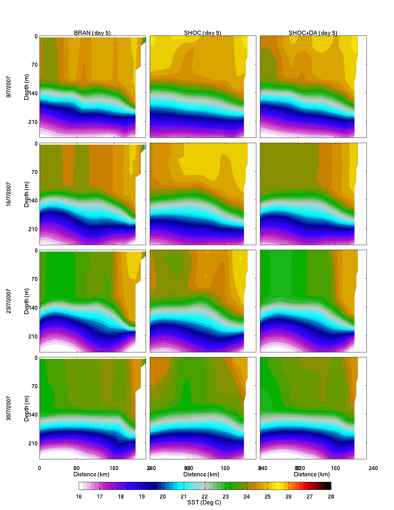
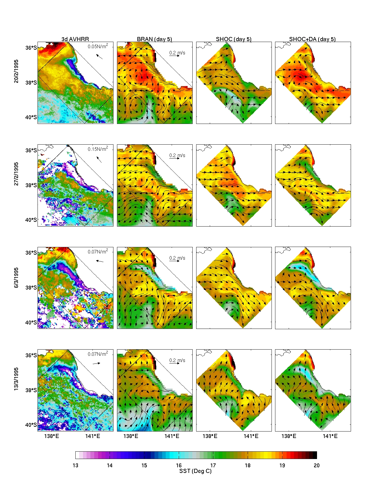
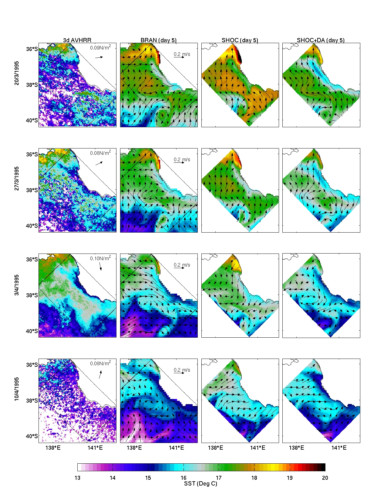
click on the images below for better resolution [~
1.1M each]
|
|
|||||||||||||||||||||||||||
|
|
Last updated 22/09/06 | Legal Notice and Disclaimer | Copyright |
|
|||||||||||||||||||||||||||