Climate change output
CSIRO Atmospheric Research Technical Paper No. 37
1998

Kevin J. Hennessy

Contents

Abstract
Background
Global climate models
Regional climate models
CSIRO climate models

Overview
CSIRO Mark 2 global climate model with slab ocean (CSIRO slab)
CSIRO regional climate model (DARLAM)
CSIRO global coupled ocean-atmosphere-sea-ice model (CSIRO coupled)

Experiments conducted
Experiment 1: CSIRO Mark 2 slab GCM 1×CO₂ and 2×CO₂ simulations
Experiment 2: DARLAM 1×CO₂ and 2×CO₂ simulations
Experiment 3: CSIRO coupled GCM transient CO₂ simulation
Output available

Value-added products

Tailored output
OzClim PC software
Licence agreement

Obtaining output
Appendix 1: CSIRO Mark 2 global climate model output
Appendix 2: CSIRO regional climate model (DARLAM) output
Appendix 3: CSIRO coupled ocean-atmosphere global climate model output

References

Acknowledgments

Abstract

The CSIRO Climate Change Research Program is Australia’s largest and most comprehensive program investigating the greenhouse effect and global climate change. This document lists the output from CSIRO climate models that have been used to conduct enhanced greenhouse experiments. Two global climate models (GCMs) and a regional climate model (RCM) are described.

Three CSIRO enhanced greenhouse experiments were undertaken. Provision of output from these experiments is intended to give other scientists an internally consistent set of detailed climatic variables for use in sensitivity studies. The first experiment was performed in 1994 with the CSIRO Mark 2 slab GCM, where enhanced greenhouse conditions were represented by an instantaneous doubling of CO₂. Output from this experiment was fed into the second experiment in 1995 which involved running a high resolution RCM over Australasia to produce more detailed information. The third experiment was performed in 1996 with the CSIRO coupled GCM which was driven by a gradually increasing CO₂ concentration scenario for 185 years.

A wide range of climatic variables was saved from each experiment at various time intervals and at various vertical levels. Broad groupings of the variables include temperature, precipitation, wind, pressure, cloud, evaporation, radiation, humidity, soil moisture, runoff, snow, sea-ice, mixing ratio, and heat flux. Many options exist for adding value to output saved from these experiments, through manipulating data to suit specific needs. The PC-based software package called OzClim enables regional scenarios of climate change to be generated for the whole or selected parts of Australia at various spatial resolutions, for any date between 1990 and 2100, where the user can select from a range of greenhouse gas emission scenarios, global climate sensitivity assumptions, and GCM or RCM patterns of climate change.

A detailed list of output from each experiment is supplied and steps required for obtaining output from CSIRO are explained.

Background

The climate model data presented in this report are a product of the CSIRO Climate Change Research Program (CCRP). The CCRP is Australia’s largest and most comprehensive program investigating the greenhouse effect and global climate change. It involves at least nine CSIRO Divisions and integrates work from researchers in other research institutes, particularly the Bureau of Meteorology, the Antarctic Research Centre, and the Cooperative Research Centre for Southern Hemisphere Meteorology.

A major component of the CCRP is a project entitled “Climate Change” which draws on work from other CCRP projects to form a basis for modelling climate change. This document lists the output from CSIRO climate models that have been used to conduct enhanced greenhouse experiments. Two global climate models (GCMs) and a regional climate model (RCM) were used.

Global climate models

A global climate model is a computer model representing the atmosphere, oceans, land and icecaps. By solving mathematical equations based upon the laws of physics, a GCM simulates the behaviour of the climate system. The model divides the planet into a number of vertical layers representing levels in the atmosphere and depths in the oceans, and divides the surface of the planet into a grid of horizontal boxes separated by lines similar to latitudes and longitudes. In this way, the planet is covered by a three-dimensional grid of boxes (Figure 1).

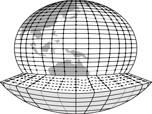
Fig 1. Schematic representation of the grid of boxes covering the Earth’s surface and atmosphere in a typical global climate model.

The horizontal size of a typical grid box in the CSIRO GCM is about 625 km by 350 km, limited largely by computer power. Inside each grid box, the mathematical equations are solved at model-timesteps of about an hour for many model-decades until a picture of the Earth’s climate is built up. Global climate models capture large scale features like the deserts and tropics very well, but have difficulty capturing smaller features like cyclones and thunderstorms because they occur at scales much smaller than the grid boxes.

Carbon dioxide (CO₂) is one of the main greenhouse gases affected by human activities. A common experiment for comparing different climate model simulations of enhanced greenhouse conditions is an instantaneous doubling of the atmospheric carbon dioxide concentration (2×CO₂). The timing of 2×CO₂ depends critically on the growth rate of greenhouse gas emissions, and the rate of uptake of CO₂ by the biosphere and oceans. The Intergovernmental Panel on Climate Change (IPCC: Houghton et al., 1996) has produced six emission scenarios which vary widely over the next century. For the mid-range scenario (IS92a), a doubling of the 1975 CO₂ concentration occurs by the year 2100. When the effects of other greenhouse gases are included, the change in radiation equivalent to a doubling of CO₂ alone occurs by the year 2060 (Dix and Hunt, 1995).

Over the ocean, most 2×CO₂ experiments use a simple “slab” of water at the lower boundary which represents the mixed-layer in the top 50 metres of ocean. Slab ocean experiments cannot take into account the potential climatic effect of changes in ocean circulation and the transfer of surface warming into the deep ocean. This is an important caveat.

Coupled ocean-atmosphere GCMs employ models of the full ocean (including the deep ocean). They can simulate the uptake of surface warming by the deep ocean and changes in ocean circulation, and the consequent effect this has on regional climate change. Some features of climate variability associated with the El Niño-Southern Oscillation (ENSO) are also captured by coupled models. In addition, coupled models are driven by a realistic IPCC scenario of steadily increasing (transient) concentrations of carbon dioxide when run under enhanced greenhouse conditions, rather than an instantaneous doubling of CO₂.

Coupled models are conceptually better than models with a slab ocean, but the choice of model for Australian studies is unfortunately not that simple. The discussion below outlines why output from both slab and coupled models should be considered equally valid, at the present time.

In the northern hemisphere, the patterns of simulated temperature and rainfall change are similar in slab and coupled models. From the perspective of regional scenario development in the northern hemisphere, the move to using coupled models is not a big issue. However, the differences are large in the southern hemisphere. Coupled models simulate a strong uptake of heat into the deep ocean in high southern latitudes, leading to reduced surface warming relative to other latitudes, whereas slab models do not show this reduction in warming. In particular, slab models simulate increased rainfall over northern and western Australia in summer, but coupled models simulate decreased rainfall (CSIRO, 1996; Whetton et al., 1997b).

There are two reasons why coupled models may be over-estimating the reduced warming in high southern latitudes. Oceanic observations suggest that the Southern Ocean is not mixed as actively as is typically simulated in coupled models (England, 1995), and observed temperature trends this century do not show a reduced warming in higher latitudes of the southern hemisphere relative to other parts of the world (Kattenberg et al., 1996). However, slab models may be over-estimating the Southern Ocean warming because they do not include uptake of heat by the deep ocean.

Therefore, coupled models may be under-estimating the warming in the Southern Ocean and slab models may be over-estimating the warming. Until the problems associated with coupled models in the southern hemisphere are resolved or at least reduced, output derived from both slab and coupled models are worth analysing for the Australian region.

Regional climate models

To improve regional detail in climate models, it is desirable to reduce the spacing between gridpoints. However, due to the complexity of global climate modelling, computational requirements become prohibitive if the horizontal grid resolution is less than a few hundred kilometres. At this resolution, vitally important small-scale phenomena, like tropical cyclones and cold fronts, are poorly captured. This affects simulated patterns of temperature and rainfall, and hence the ability to realistically simulate observed regional climate features in GCMs.

A computationally feasible alternative to a coarse resolution global climate model is to use a finer resolution model over a small part of the globe. A regional climate model (RCM), with a horizontal resolution of about 100 km or less, is able to simulate regional weather patterns better than most GCMs (McGregor et al., 1993). Part of the reason for the improved climate simulation relative to GCMs is the fact that coastlines and mountains are represented in more detail in RCMs. Since topographic features strongly influence regional temperature and rainfall, more detailed features are likely to give a better climate simulation.

A regional climate model requires weather information at its lateral boundaries in order to simulate weather within its boundaries. For climate change studies, an RCM is typically driven at its boundaries by information from a coarser-scale GCM. This is commonly called nesting an RCM inside a GCM. One-way nesting allows information to flow from the GCM to the RCM each simulated day, but the weather simulated by the RCM does not affect the GCM interactively. This means that the RCM can be run after the GCM experiment has been completed.

The application of RCMs to decadal-scale climate modelling is only recent, since RCMs have mainly been used in the past for short-term weather forecasting. Very few RCMs have been used for climate change experiments, and CSIRO is a leader in this field. Although the performance of an RCM is constrained by its reliance on GCM performance at the lateral boundaries, RCMs offer detailed insight into regional climate change. The ability to use fine resolution RCM climate change output should be seen as a significant opportunity.

CSIRO climate models

Overview

This section describes the three CSIRO climate models used in enhanced greenhouse experiments. There are two coarse resolution global climate models and a fine resolution regional climate model. Since each model was developed at CSIRO, there are many similarities.

Each model uses the same basic equations which describe the laws of physics. Schemes for boundary layer mixing, moisture advection, radiation and cloud formation are also common to each model. The simulation of average climate for selected variables has been validated against observed average climatic data as part of standard model testing procedures. Simulations described in this report are from models which have passed global and Australian climate validation, so that some confidence may be placed in output from enhanced greenhouse simulations, taking the following caveats into account.

The models do not (and cannot) take into account all processes (natural and anthropogenic) which affect climate variability and change. Some processes are not well understood and others must be represented in a simplified way in order to ensure computational efficiency. While continental-scale climatic features are well simulated for present conditions, regional features are captured with less accuracy.

None of the models includes the regional cooling effect of sulfate aerosol which has been identified by the IPCC (Houghton et al., 1996) as an important element of anthropogenic climate change, particularly in the northern hemisphere where aerosol are emitted in large quantities. While aerosol emissions in Australia are relatively small, northern hemisphere aerosol may influence the Australian climate indirectly, through long-distance climatic teleconnection patterns (e.g. the influence of Asian aerosols on land-sea temperature gradients which may affect the Australian monsoon).

Simplifications in the representation of ocean processes are likely to be important in determining patterns of climate change in the Australian region, such as changes in the vertical profile of ocean temperature/salinity and the El Niño - Southern Oscillation. The climatic influence of small-scale features such as tropical cyclones and storms cannot be resolved at this stage.

Plant physiology is not included, so simulated vegetation does not respond to climate change or increased levels of CO₂. However, significant biospheric responses to climate change could occur in the real world, as could changes in land-use, with consequent climatic feedbacks.

CSIRO Mark 2 global climate model with slab ocean (CSIRO slab)

The CSIRO Mark 2 GCM is a spectral model with R21 horizontal resolution (grid boxes measuring about 625 km by 350 km) and has 9 vertical levels in the atmosphere (Watterson et al., 1997). This gives 41 grid boxes over Australia. Global atmospheric and biospheric sub-models are coupled to a slab ocean sub-model. Simplifications of physical processes such as convection, radiation, gravity wave drag, cloud formation, sea-ice formation and biospheric interactions are detailed in McGregor et al. (1993), McGregor (1993), Kowalczyk et al. (1994) and O’Farrell (1998).

Adjusted heat fluxes are applied to the slab ocean to represent heat from the deep ocean and the effect of currents (Watterson et al., 1997). Fluxes are determined from a separate 10-year experiment driven by observed sea-surface temperatures (SSTs). Regional flux adjustments are required to keep simulated sea-surface temperatures close to those observed, and these monthly average flux adjustments were saved for use in 1×CO₂ and 2×CO₂ experiments. When flux adjustments are applied in the 1×CO₂ run, the simulated SSTs and other continental-scale climatic features are similar to those observed. The same flux adjustments are applied in the 2×CO₂ run, which places an artificial constraint on the variability of sea-surface temperature as the climate changes. This limitation may have important implications for projected ocean behaviour and atmospheric circulation patterns. On a CRAY Y-MP computer, climate variables for one model day take 30 seconds to evaluate, so a 10 year run takes 50 hours.

CSIRO regional climate model (DARLAM)

Over the Australasian region (71°E–177°E, 12°N–57°S), the CSIRO regional climate model (DARLAM) has been driven at its lateral boundaries by output from the CSIRO Mark 2 GCM (Walsh and McGregor, 1995; McGregor et al., submitted). DARLAM has nine vertical levels in the atmosphere and grid boxes measuring about 125 km by 125 km, giving 442 grid boxes over Australia (Figure 2).

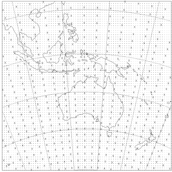
Fig 2. DARLAM model domain for simulations using a 125 km grid (dots). Gaussian gridpoints of the R21 CSIRO slab GCM are indicated by crosses (from Walsh and McGregor, 1995).

The atmospheric sub-model interacts with a slab ocean sub-model and uses descriptions of physical processes which are similar to those in the CSIRO Mark 2 GCM. However, DARLAM uses a modified convection scheme, a different soil moisture scheme and excludes gravity wave drag. Sensitivity experiments showed that results were not greatly affected by the change in convection scheme. On a CRAY Y-MP computer, climate variables for one model day take 130 seconds to evaluate, so a 10 year run takes 132 hours.

CSIRO global coupled ocean-atmosphere-sea-ice model (CSIRO coupled)

The CSIRO coupled model involves global atmospheric, oceanic, sea-ice and biospheric sub-models (Gordon and O'Farrell, 1997; Hirst et al., 1997). The atmospheric, biospheric and sea-ice sub-models are the same as those used in the CSIRO Mark 2 GCM. Atmospheric and oceanic components use a spectral R21 horizontal grid (each gridbox measuring about 625 km by 350 km) with 9 vertical levels in the atmosphere and 21 levels in the ocean. The ocean model has a heat transport scheme which significantly reduces problems associated with excessive mixing in the Southern Ocean. On a CRAY Y-MP computer, climate variables for one model day take 60 seconds to evaluate, so a 10 year run takes 61 hours.

Coupling the atmosphere to the ocean is technically challenging because the ocean has a much longer timescale of variability than the atmosphere. The coupled model requires adjustments to the fluxes of heat, salinity and wind stress which link the atmospheric and oceanic components. Adjusting the heat fluxes at the ocean/atmosphere/ice interface is performed by running the ocean and atmosphere models independently and computing (i) the fluxes required by the ocean model when driven by observed SST, sea-surface surface salinity (SSS) and wind stress, and (ii) the heat fluxes generated by the atmosphere/ice model with observed SST and SSS. The flux adjustment is the difference between (i) and (ii). These adjustments were used in the fully coupled model which generates its own SST, SSS and wind stress.

The same flux adjustments are applied to the transient CO₂ run (Hirst et al., 1997), which places an artificial constraint on the variability of sea-surface temperature as the climate changes. Flux adjustments in the coupled experiment are much smaller than the Q-fluxes in the CSIRO slab experiment.

Experiments conducted

This section describes three CSIRO enhanced greenhouse experiments. Provision of output from these experiments is intended to give users an internally consistent set of detailed climatic variables for use in sensitivity studies. Those wishing to undertake impact assessments or sensitivity studies which incorporate a wider range of future climates should use the simplified scenarios of CSIRO (1996) which are based on consensus results of five international global climate models.

The first experiment described below was performed in 1994 with the CSIRO Mark 2 slab GCM, where enhanced greenhouse conditions were represented by an instantaneous doubling of CO₂. Output from this experiment was fed into the second experiment in 1995 which involved running a high resolution regional climate model over Australasia to produce more detailed information. The third experiment was performed in 1996 with the CSIRO coupled GCM which was driven by a gradually increasing CO₂ concentration scenario for 185 years.

Other experiments have been performed and new experiments are planned. Data sets described below are those which have been checked and published in peer-reviewed literature. Researchers should ask whether more recent data sets have been made available since the publication of this document. More information can be obtained from Dr Roger Jones.

Experiment 1: CSIRO Mark 2 slab GCM 1×CO₂ and 2×CO₂ simulations

In the control experiment, the model was run for 30 model-years of 1×CO₂ conditions (an atmospheric concentration of 326 parts per million (ppm) from the year 1973). In the enhanced greenhouse experiment, the model was run for 55 years of 2×CO₂ conditions (660 ppm), and the global mean temperature reached equilibrium during the last 30 years. For a doubling of CO₂, the global mean warming at equilibrium is 4.3°C (Figure 3).

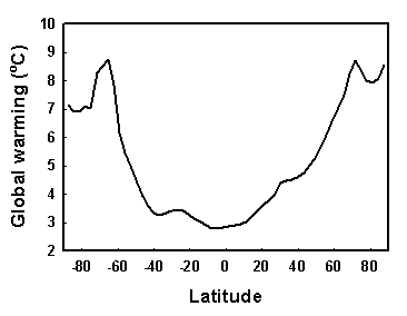
Fig 3. Zonal and annual mean change in surface temperature for a doubling of CO₂ from 330 ppm to 660 ppm in the CSIRO slab GCM (from Watterson et al., 1997).

The climate variables saved are listed in Appendix 1.

Experiment 2: DARLAM 1×CO₂ and 2×CO₂ simulations

Over the Australasian region (71°E–177°E, 12°N–57°S), DARLAM has been driven at its lateral boundaries by output from the CSIRO Mark 2 GCM for 20 years of 1×CO₂ and 2×CO₂ conditions (McGregor et al., submitted). Observed precipitation and temperature are much better simulated in DARLAM than in the CSIRO Mark 2 GCM (Figure 4), largely because DARLAM captures topographic effects not able to be represented in the GCM. Under 2×CO₂ conditions, DARLAM simulated patterns of precipitation and temperature change which can differ significantly from those simulated by the host GCM (Whetton et al., 1997a).

Fig 4. Atmospheric CO₂ concentration (parts per million - ppm) used in the CSIRO coupled GCM for IS92a transient CO₂ simulations (from Hirst et al., 1997).

The climate variables saved are listed in Appendix 2.

In more recent simulations, DARLAM has been run at 60 km resolution over south-eastern Australia (Whetton et al., 1997a, b), New Zealand, South Africa and south-east Asia. New simulations are planned at this resolution over different regions including Queensland and the south Pacific.

Experiment 3: CSIRO coupled GCM transient CO₂ simulation

The coupled model has been driven by the IPCC IS92a CO₂ scenario which increases concentrations at a rate of 0.5% per year for the first 100 years, and slightly faster thereafter (Hirst et al., 1997, Fig. 4). This scenario represents the IPCC’s “central estimate” based upon a range of assumptions about future population and economic growth, and energy supplies in the absence of climate policies beyond those already adopted. Radiative effects of changes in other greenhouse trace gases are excluded, but will be included in future experiments. The reference CO₂ concentration is 330 parts per million (ppm) for the year 1975. After 130 years the CO₂ concentration doubles to 660 ppm, and trebles after 180 years. At the time of 2×CO₂, the global mean warming of near-surface air is 2.2°C, and at 3×2 the warming is 3.8°C (Fig. 5). This is about half the warming generated by Experiments 1 and 2, largely due to the greater uptake of heat by the deep ocean in the coupled model which results in less warming near the surface.

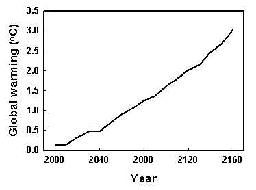
Fig 5. The global mean change (IS92a-1×CO₂) in surface temperature (oC) simulated by the CSIRO coupled GCM (from Hirst, 1996).

The climate variables saved from the coupled GCM experiment are listed in Appendix 3.

Output available

A wide range of climatic variables have been saved from each experiment at various time intervals and at various vertical levels. Broad groupings of the variables include:

• temperature
• precipitation
• wind
• pressure
• cloud
• evaporation
• radiation
• humidity
• soil moisture
• runoff
• snow
• sea-ice
• mixing ratio
• heat flux

In Experiment 1 (CSIRO slab GCM), for 30 years of both 1×CO₂ and 2×CO₂ conditions, 38 variables were saved at 8-hourly intervals, 13 variables were saved 24-hourly, and 95 variables were saved as monthly averages (Appendix 1).

In Experiment 2 (DARLAM), for 20 years of both 1×CO₂ and 2×CO₂ conditions, 13 variables were saved at 3-hourly intervals, 51 variables were saved 12-hourly, 2 variables were saved 24-hourly, and 51 variables were saved as monthly averages (Appendix 2).

In Experiment 3 (CSIRO coupled GCM), for 185 years of transient CO₂ conditions, 98 atmospheric variables and 108 oceanic variables were saved as monthly averages (Appendix 3).

Value-added products

Tailored output

The output listed in Appendices 1, 2 and 3 may not suit the applications of all users. CSIRO is open to negotiation about supplying alternative products that are tailored to meet specific needs. For example:

• users may want variables which were not saved, but can be derived from a combination of saved variables (e.g. dewpoint temperature).
• in some cases the model may be re-run to provide different variables or higher temporal resolution
  users may want long-term (multi-year) averages of particular variables, rather than many years of daily or monthly data
• regionally-specific subsets of the data may suit users with limited geographical interest or limited data storage facilities
• output in the form of maps or graphs can also be produced
• data scaled for particular years in the future, taking into account different greenhouse gas emission scenarios, different sulphate aerosol emission scenarios, different global climatic sensitivities to changes in greenhouse gas concentrations, and different patterns of climate change simulated by various climate models (see OzClim below).

Many other possibilities exist for adding value to output saved from CSIRO climate change experiments. CSIRO supplied out put to over 40 collaborative projects from 1990 to 1995 (Hennessy et al., 1995) and output to a further 20 collaborative projects from 1995-1997 Collaboration in scenario development and impact projects 1990-97). Where possible, supply of value-added data will be free of charge, particularly for funded collaborative projects.

OzClim PC software

CSIRO and the International Global Change Institute (IGCI), University of Waikato (New Zealand) have developed a PC-based software package called OzClim which runs under Microsoft Windows 95. OzClim enables regional scenarios of climate change to be generated for the whole or selected parts of Australia at various spatial resolutions, for any date between 1990 and 2100 (Jones, 1996; Collaboration in scenario development and impact projects 1990-97). The user can select from a range of greenhouse gas emission scenarios, global climate sensitivity assumptions, and GCM or RCM patterns of climate change.

The advantage of this approach is that the effect of a range of options, assumptions or policy measures can be explored in an internally consistent way, and the effects of uncertainty can be calculated explicitly. The system will also allow easy updating as new scenario information becomes available. This will be necessary as sulfate aerosol and ozone depletion effects are incorporated into climate models. Output is displayed in the form of colour maps and graphs (Fig 6).

It is planned to couple OzClim with a GIS database, and with various impact models for sectors such as agriculture, ecosystems and hydrology. The integrated system will also be capable of use for climate variability studies using historical climate data sets.

Disclaimer

Obtaining output

The first point of contact regarding access to CSIRO climate change output is through the Climate Impact Liaison Officer, Dr Roger Jones, at CSIRO Division of Atmospheric Research. Output can be provided in a range of formats or grid resolutions to suit different applications, and can be supplied on Exabyte / DAT media or transferred between computers via FTP.

As part of the Climate Change Research Program, the Climate Change Impacts and Adaptation Project also co-ordinates a great deal of information on climate change impacts research in Australia. This is available on request through Dr Jones.

Inquiries about specific aspects of the climate change experiments, information about forthcoming experiments, requests for alternative variables to be saved in new experiments, or requests for material cited in this report can also be directed through Dr Jones, whose contact details are:

Dr Roger Jones
CSIRO Division of Atmospheric Research
Private Bag No. 1
Aspendale, Victoria, Australia, 3195
Ph +61 3 9239 4555
Fax +61 3 9239 4444
E-mail roger.jones@csiro.au

Appendix 1

CSIRO9 Mark 2 global climate model output

1×CO₂ & 2×CO₂ experiments
30 year timeseries
(350 km × 625 km resolution over the globe)

‡ Data for 9 atmospheric sigma levels (L×surface pressure, where L = 0.979, 0.914, 0.803, 0.670, 0.500, 0.340, 0.197, 0.086 and 0.021)

8-hourly data:

• Moisture mixing ratio ‡
• Pressure at surface
• Temperature ‡
• Temperature at surface
• Wind speed: meridional (south–>north) ‡
• Wind speed: zonal (west–>east) ‡

24-hourly data

(* = average of 48 half-hourly values):

• Cloud fraction: total *
• Evaporation: potential and actual *
• Precipitation: convective and *
• Pressure: sea-level
• Radiation: downward shortwave at surface *
• Radiation: net longwave at top of atmosphere *
• Relative humidity at 2m above surface *
• Soil moisture in lowest layer (28.5–278.5 cm below surface)
• Soil moisture in middle layer (3–28.5 cm below surface)
• Temperature at 2m above surface *
• Temperature at surface *
• Temperature: max & min at 2m above surface
• Wind speed at 10m above surface *

Monthly-mean data

• Albedo
• Cloud fraction: low level, middle level, high level, total
• Evaporation: potential and actual
• Heat flux: latent ‡
• Heat flux: sensible at surface
• Ice concentration
• Ice-ocean heat flux
• Ice-ocean salt flux
• Moisture mixing ratio ‡
• Precipitation: total, convective, canopy interception
• Pressure: sea-level
• Radiation: clear sky longwave out at top of atmosphere
• Radiation: clear sky net longwave at surface
• Radiation: clear sky net shortwave at surface
• Radiation: clear sky shortwave out at top of atmosphere
• Radiation: downward longwave at surface
• Radiation: downward shortwave at surface
• Radiation: longwave out at top of atmosphere
• Radiation: net longwave at surface
• Radiation: net shortwave at surface
• Radiation: shortwave out at top of atmosphere
• Relative humidity at 2m above surface
• Runoff
• Sea-ice depth
• Snow depth
• Soil moisture in lowest layer (28.5–278.5 cm below surface)
• Soil moisture in middle layer (3.0–28.5 cm below surface)
• Temperature ‡
• Temperature: max, min, mean at surface (bare soil)
• Temperature: max, min, mean at surface (vegetated)
• Temperature of lowest soil layer (28.5–278.5 cm below surface)
• Temperature of middle soil layer (3.0–28.5 cm below surface)
• Temperature: extreme monthly max and min at 2m above surface
• Temperature: max, min, average at 2m above surface for bare ground and canopy
• Wind speed at surface
• Wind speed: meridional (south–>north) ‡
• Wind speed: zonal (west–>east) ‡
• Wind stress: meridional (south–>north) at surface
• Wind stress: zonal (west–>east) at surface

Note
Other variables not listed here and timeseries-averages can be derived from archived data upon request.

Appendix 2

CSIRO regional climate model (DARLAM) output

1×CO₂ & 2×CO₂ experiments
10 year timeseries
(125 km resolution over Australasia (71 °E–177 °E, 12 °N–57 °S))

‡ Data for 9 atmospheric sigma levels (L×surface pressure, where L = 0.979, 0.914, 0.803, 0.670, 0.500, 0.340, 0.197, 0.086 and 0.021)

3-hourly data:

• Cloud fraction: total
• Heat flux: latent at surface
• Heat flux: sensible at surface
• Radiation: clear sky net shortwave at surface
• Radiation: downward longwave at surface
• Radiation: net shortwave at ground
• Radiation: shortwave at top of atmosphere
• Relative humidity at 2m above surface
• Temperature at surface
• Temperature at 2m above surface
• Wind speed at 2m above surface
• Wind speed at 3m above surface
• Wind speed at 10m above surface
  

12-hourly data:

• Cloud fraction: low, middle, high
• Moisture mixing ratio ‡
• Precipitation: total, convective
• Pressure at surface
• Radiation: clear sky longwave at top of atmosphere
• Radiation: long wave at top of atmosphere
• Runoff
• Soil moisture in lower layer (0–100 cm below surface)
• Temperature ‡
• Temperature at surface
• Temperature of middle soil layer (3.0–28.5 cm below surface)
• Temperature of lowest soil layer (28.5–278.5 cm below surface)
• Wind speed: meridional (south–>north) ‡
• Wind speed: zonal (west–>east) ‡
• Wind stress: meridional (south–>north) at surface
• Wind stress: zonal (west–>east) at surface

24-hourly data:

• Temperature: max & min at 2m above surface

Monthly-mean data:

• Cloud fraction: low, middle, high
• Moisture mixing ratio ‡
• Precipitation: total, convective
• Pressure at surface
• Radiation: clear sky longwave at top of atmosphere
• Radiation: long wave at top of atmosphere
• Runoff
• Soil moisture in lower layer (0–100 cm below surface)
• Temperature ‡
• Temperature at surface
• Temperature of middle soil layer (3.0–28.5 cm below surface)
• Temperature of lowest soil layer (28.5–278.5 cm below surface)
• Wind speed: meridional (south–>north) ‡
• Wind speed: zonal (west–>east) ‡
• Wind stress: meridional (south–>north) at surface
• Wind stress: zonal (west–>east) at surface

Note
Other variables not listed here and timeseries-averages can be derived from archived data upon request.

Appendix 3

CSIRO9 global coupled ocean-atmosphere climate model output

IPCC IS92a CO₂ experiment
185 year timeseries
(350 km × 625 km resolution over the globe)

‡ Data for 9 atmospheric sigma levels (L×surface pressure, where L = 0.979, 0.914, 0.803, 0.670, 0.500, 0.340, 0.197, 0.086 and 0.021)

ß Data for 21 oceanic levels at depths of 12.5, 37.5, 65, 98.5, 138.5, 185, 240, 310, 410, 545, 710, 905, 1130, 1395, 1720, 2125, 2575, 3025, 3475, 3925, 4375 metres below surface

Monthly-mean data

• Albedo
• Cloud fraction: low level, middle level, high level, total
• Evaporation: potential and actual
• Heat flux: latent ‡
• Heat flux: sensible at surface
• Freshwater flux at ocean surface
• Ice concentration
• Ice-ocean heat flux
• Ice-ocean salt flux
• Moisture mixing ratio ‡
• Ocean current velocity: meridional (south–>north)ß
• Ocean current velocity: zonal (west–>east) ß
• Ocean current velocity: vertical ß
• Oceanic streamfunction ß
• Precipitation: total, convective, canopy interception
• Pressure: sea-level
• Radiation: clear sky longwave out at top of atmosphere
• Radiation: clear sky net longwave at surface
• Radiation: clear sky net shortwave at surface
• Radiation: clear sky shortwave out at top of atmosphere
• Radiation: downward longwave at surface
• Radiation: downward shortwave at surface
• Radiation: longwave out at top of atmosphere
• Radiation: net longwave at surface
• Radiation: net shortwave at surface
• Radiation: shortwave out at top of atmosphere
• Relative humidity at 2m above surface
• Runoff
• Salinity ß
• Sea-ice depth, west–>east velocity, south–>north velocity
• Snow depth
• Soil moisture in upper layer (3.0–28.5 cm below surface)
• Soil moisture in lower layer (28.5–278.5 cm below surface)
• Soil percolation
• Temperature ‡,ß
• Temperature: max, min, mean at surface (bare soil)
• Temperature: max, min, mean at surface (vegetated)
• Temperature of middle soil layer (3.0–28.5 cm below surface)
• Temperature of lowest soil layer (28.5–278.5 cm below surface)
• Temperature: extreme monthly max and min at 2m above surface
• Temperature: max, min, average at 2m above surface for bare
• ground and canopy
• Wind speed at surface
• Wind speed: meridional (south–>north) ‡
• Wind speed: zonal (west–>east) ‡
• Wind stress: meridional (south–>north) at surface
• Wind stress: zonal (west–>east) at surface

Note
Other variables not listed here and timeseries-averages can be derived from archived data upon request.

References

CSIRO (1996): Climate change scenarios for Australia. CSIRO Division of Atmospheric Research, 8 pp.

Dix, M.R. and Hunt, B.G. (1995): Climatic modelling — doubling of CO₂ levels and beyond. Final report to the Federal Department of the Environment, Sport and Territories. CSIRO Division of Atmospheric Research, 28 pp.

England, M.H. (1995): Using chlorofluorocarbons to assess ocean climate models, Geophys. Res. Lett., 22 (22), 3051–3054.

Gordon, H.B. and O'Farrell, S.P. (1997) Transient climate change in the CSIRO coupled model with dynamic sea ice. Monthly Waether Review, 125(5), 875–907.

Hennessy, K.J., Whetton, P.H. and Pittock, A.B. (1995) CSIRO Climate Change Research Program: Collaboration in Scenario Development and Impact Projects 1990–1995. CSIRO Division of Atmospheric Research Report, 51 pp.

Hirst, A.C., Gordon, H.B. and O’Farrell, S.P. (1997): Response of a coupled ocean-atmosphere model including oceanic eddy-induced advection to anthropogenic CO₂ increase. Geophys. Res. Lett., 23(23), 3361–3364.

Houghton, J.T., Meira Filho, L.G., Callander, B.A., Harris, N., Kattenberg, A. and Maskell, K. (eds.), Climate Change 1995, The Science of Climate Change. Contribution of Working Group 1 to the Second Assessment Report of the IPCC, Cambridge University Press, 572 pp.

Jones, R.N. (1996): OzClim — A Climate Scenario Generator and Impacts Package for Australia. CSIRO Division of Atmospheric Research.

Kattenberg, A, Giorgi, F., Grassl, H., Meehl, G.A., Mitchell, J.F.B., Stouffer, R.J., Tokioka, T., Weaver, A.J. and Wigley, T.M.L. (1996): Climate models — projections of future climate. In: J.T. Houghton, L.G. Meira Filho, B.A. Callander, N. Harris, A. Kattenberg, and K. Maskell (eds.), Climate Change 1995, The Science of Climate Change. Contribution of Working Group 1 to the Second Assessment Report of the IPCC, Cambridge University Press, 285–358.

Kowalczyk, E.A., Garratt, J.G. and Krummel, P.B. (1994): Implementation of a soil-canopy scheme into the CSIRO GCM — regional aspects of the model response. Technical Paper 32, CSIRO Division of Atmospheric Research.

McGregor, J.L. (1993): Economical determination of departure points for semi-Lagrangian models. Mon. Wea. Rev., 121, 221–230.

McGregor, J.L., Walsh, K.J. and Katzfey, J.J. (1993): Nested modelling for regional climate studies. In: A.J. Jakeman, M.B. Beck and M.J. McAleer (eds.), Modelling Change in Environmental Systems, J. Wiley and Sons, 367–386.

McGregor, J.L., Katzfey, J.J. and Nguyen, K.C. (submitted): Seasonally-varying nested climate simulations over the Australian region. J. Climate.

O’Farrell, S.P. (1998): Investigation of the dynamic sea-ice component of a coupled atmosphere sea-ice general circulation model. J. Geophys. Res. (in press)

Walsh, K.J. and McGregor, J.L. (1995): January and July climate simulations over the Australian region using a limited-area model. J. Climate, 8 (10), 2387–2403.

Watterson I.G., O’Farrell, S.P. and Dix M.R. (1997): Energy transport in climates simulated by a GCM which includes dynamic sea-ice. J. Geophys. Res., STRONG>102(D10), 11027–11037.

Whetton, P.H., Katzfey, J.J., Nguyen, K., McGregor, J.L., Page, C.M., Elliot, T.I. and Hennessy, K.J. (1997a): Fine Resolution Climate Change Scenarios for New South Wales - Part 2: Climate Variability CSIRO 1996-1997 Consultancy Report for NSW Environment Protection Authority, 51 pp.

Whetton, P.H., Wu, X., McGregor, J.L., Katzfey, J.J. and Nguyen, K. (1997b): Fine Resolution Assessment of Enhanced Greenhouse Climate Change in Victoria. CSIRO Consultancy Report. Victorian Environment Protection Authority Publication 574, 34 pp.

Acknowledgments

The climate model data resources listed in this report have been made available by the efforts of many climate modellers and data analysts in CSIRO Climate Change Research Program.

Funding for the generation and analysis of CSIRO climate change data is provided by the National Greenhouse Research Program via the Federal Department of the Environment, Sport and Territories, the Governments of Victoria, New South Wales, Queensland, the Northern Territory and Western Australia, and CSIRO.

Comments from Dr Chris Mitchell, Dr Barrie Pittock and Dr Roger Jones of CSIRO Division of Atmospheric Research were very useful.

Data listings from Mr Martin Dix and Dr Jack Katzfey of CSIRO Division of Atmospheric Research are particularly appreciated.

This work is a product of the CSIRO Climate Change Research Program. The document was written by Kevin Hennessy and the electronic version compiled by Roger Jones.

Back to Climate Impact Group

Modified: April 3, 2008