Slide 1 of 20

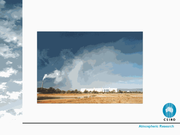
Dispersion modelling is needed to assess a population's risk of exposure to air pollution from local sources. A dispersion model describes the transport and diffusion of pollutants in the atmosphere. An example of the use of dispersion modelling is the assessment of the effect of a power station plume on a nearby town. Worst-case concentrations of pollutants can be estimated in various parts of the town, the general effect of the main chemical transformations can be conservatively estimated and an assessment of the population risk to exposure can be made. Common assumptions in simple dispersion models include very simple meteorology, simple representation of the effects of terrain and no chemical transformations.

Slide 2 of 20

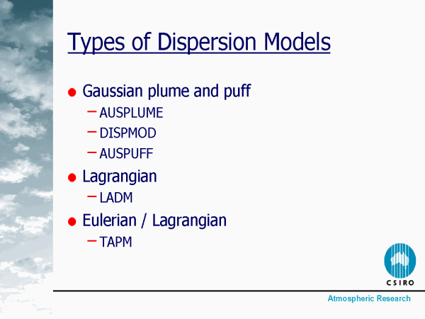
Types of dispersion models include Gaussian plume, puff and Lagrangian models. Regulatory models are of the former type. In this presentation, these models, the data requirements and outputs from some commonly used Australian models will be briefly described.

Slide 3 of 20

• Scales of modelling and applications
  • urban area (whole airshed - see the presentation on Urban-Scale Air Pollution Models) versus local point source study (assess the effect of a power station plume on a nearby town)
  • dispersion models - modelling a local source or sources with the prime interest in the region close to the source (near source ground level concentrations)
  • statistical output rather than specific time and place

• Assumptions: simple meteorology, no complex terrain, no chemical transformations
  • common assumptions include simple met, simple representation of the effects of terrain (no complex terrain) and no chemical transformations
  • often their underlying assumptions are not valid at larger scales; sea-breezes, valley flows, recirculation of air (polluted/clean)

• Fast turnaround - regulatory work

• run relatively quickly on PC and are often used for regulatory work

Slide 4 of 20

Example of use of dispersion modelling is assessment of the effect of a power station on a nearby town.

Slide 5 of 20

• Types of (Australian) dispersion models
  • include Gaussian plume, puff and Lagrangian
    • Most widely used models for predicting the impact of relatively non-reactive gases, like SO₂, released from stacks, are based on Gaussian diffusion. Spread of a plume in vertical and horizontal is assumed to occur by simple diffusion along the direction of the mean wind. They have been widely used because they don’t need to be run on a supercomputer. (Regulatory models often lag current research because of delays in validating new approaches.)
  • AUSPLUME (Gaussian regulatory model)
  • DISPMOD (regulatory model, Gaussian plume and shoreline fumigation)
  • AUSPUFF (Gaussian puff model)
  • LADM (Lagrangian model)
  • TAPM (Lagrangian and Eulerian - has features like relatively fast turnaround)

Slide 6 of 20

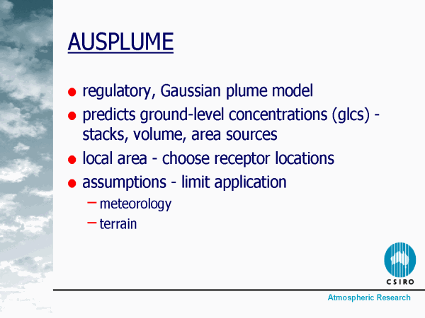
• AUSPLUME - Australian regulatory model
  • Gaussian plume dispersion model
    • based on the premise that cross-sections through elevated plumes from point sources have Gaussian distribution of concentration
    • instantaneous snap-shots of plumes generally not consistent with this image but experiments show if averaged over long enough time or many experiments, mean distribution is close to Gaussian.
    • Dispersion coefficients. Most are functions of stability and distance downwind from the source
  • predicts ground-level concentrations (GLCs) from one or more sources - stacks, area, volume
  • generally used area of up to few 100s of square kms around sources, user chooses where to calculate ground level concentrations (receptor points) - doesn’t have to be a grid.
  • simplifying assumptions (limit where it should be applied)
    • simple meteorology (no horizontal variation) to transport and diffuse pollutants. Winds same at every receptor point for a particular hour with the pollutant transported in ‘straight lines’ from source to receptor. Winds and diffusion are independent from one hour to next. No modelling of recirculation due to sea-breeze etc.
    • flat, near flat terrain
    • valid where terrain is flat or near flat and where there is little horizontal variation in the winds (eg. Not mountainous regions, coastal regions, etc.) often used in these sits
    • Doesn’t allow for chemical transformations

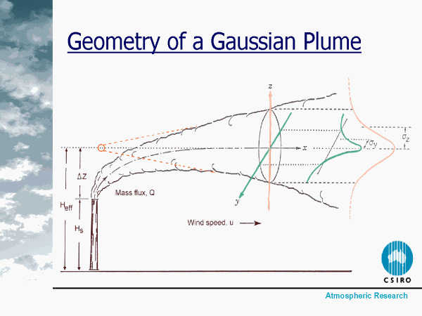
Slide 7 of 20

Plume cross-section, showing how AUSPLUME models the plume

Slide 8 of 20

• DISPMOD
  • Gaussian plume dispersion model but also capable of simulating shoreline fumigation
    • plume released at a coastal location may be in stable air above the thermal internal boundary layer (TIBL) and subject to little vertical dispersion
    • TIBL grows with distance inland, as plume travels inland it may intersect the TIBL and fumigate

• DISPMOD models ground-level concentrations resulting from fumigation and dispersion
• The most significant feature of the model is its capability to simulate shoreline fumigation
• As for AUSPLUME, it is not capable of handling complex wind flows or recirculating pollutants

Slide 9 of 20

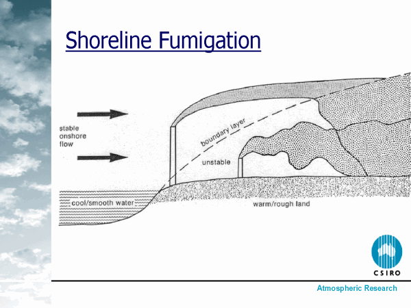
Shoreline fumigation modelled by DISPMOD

• plume released at a coastal location may be in stable air above the thermal internal boundary layer and subject to little vertical dispersion
• TIBL grows with distance inland, as plume travels inland it may intersect the TIBL and fumigate

Slide 10 of 20

AUSPUFF

• non-steady-state Gaussian puff model - was designed to become a regulatory model
• unlike AUSPLUME, it can be used in conditions with complex meteorology - requires 3-D met data set (diagnostically (AUSMET), or prognostically from CSUMM model supplied with AUSPUFF)
• would take a very long time to run the meteorological program CSUMM for a year
• in situations where winds vary with time but not horizontally, it can be used with a simpler AUSPLUME met file. Then AUSPUFF can represent recirculation of pollutants by continuously releasing and following puffs
• can handle simple chemical transformation explicitly

Slide 11 of 20

• Gaussian Models
  • no chemical transformations (AUSPUFF does include a simple, explicit chemical transformation algorithm)
  • if major chemical processes are important (e.g. oxidation of NO by O3 to form NO2), these may be estimated crudely after a model run

• Building wakes
  • some of these models include this - can be important for local problems
  • e.g. use this information when assessing impacts at proposed sites to increase stack height or move stacks away from buildings
  • need general information about set-up of proposed site

Slide 12 of 20

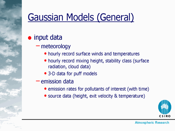
AUSPLUME - Australian regulatory model

• input data requirements
• meteorology
  • meteorology - simple hourly file (create for yourself from observations), or more complex met file - from a prognostic or diagnostic meteorological model.
  • hourly record surface winds and temperatures
  • hourly record mixing height, stability class (surface radiation, cloud)
  • there are standard AUSPLUME meteorological files (worst-case meteorology)
• emission data
  • emission rates for pollutants of interest with time variation - get this info from source, EPAs, literature, etc
  • data about sources, eg. height, diameter, exit velocity and temperature if buoyant plume
  • variation - often emission info is one of the largest sources of error (it may not matter what type of model you use)

Slide 13 of 20

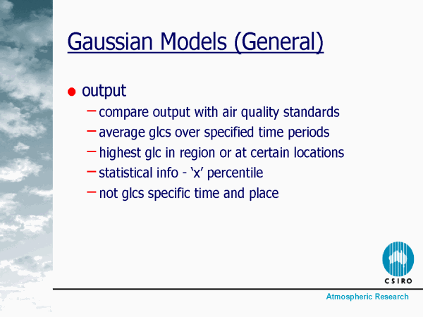
• Simple Gaussian models are often used to predict glcs over periods of up to a year or two

• Models designed to output various quantities that are generally required for comparison with air quality standards
  • averaged concentrations of pollutants over specified time periods
  • highest glc for a pollutant over a region or at certain locations within the region
  • statistical info - ‘x’ percentile (x% of the values are below the ‘x’ percentile)

• Models not used to predict glc info at a specific time and place - average quantities
  • can predict ensemble average concentration but not the transient peaks caused by downdrafts in thermal convection eddies

• To use output for population exposure work it is important to be mindful of the model assumptions, and consider the circumstances under which the models are being applied (meteorology and region)

Slide 14 of 20

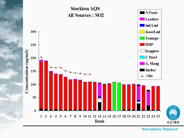
• Gaussian models- general output
• DISPMOD
  • SO2 - 1 year run
  • highest 25 hourly values cf obs for Stockton air quality station coded by source
  • Newcastle (Kooragang Island work 1992)

Slide 15 of 20

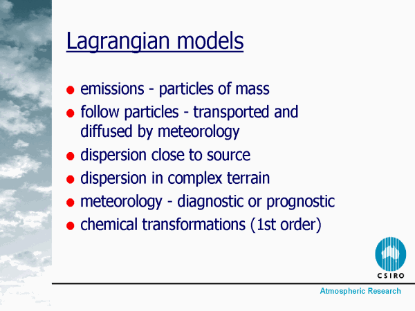
Lagrangian models

• approximate emissions as particles or puffs of mass and follow the particles as they are transported and effected by meteorology
• useful describing dispersion v. close to source or in complex topography. Re-circulation, sea breeze, valley flows, etc.
• meteorology may be run earlier or in parallel
• sophisticated versions of these models may become computer intensive as number of sources increases - can restrict their usage
• may contain chemistry formulations, generally only first-order chemistry

Slide 16 of 20

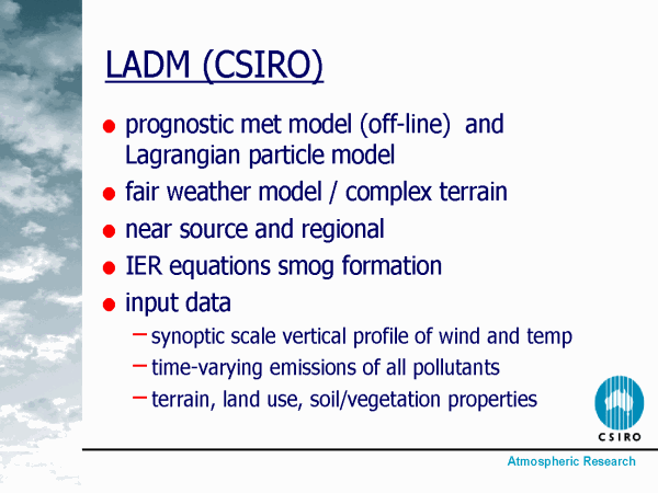
LADM - CSIRO Atmospheric Research model

• sophisticated Lagrangian model.
• meteorology is run separately with no feedback between meteorology and chemistry
• in its simplest form, LADM simulates the dispersion of non-reactive gases like SO2 and total nitrogen oxides
• LADM also includes IER equations of smog formation, and, therefore, it can model photochemical formation and dispersion of gases such as O3 and NO2 (cf Eulerian models) (click here for on-line smog calculations using the IER method)
• ‘fair-weather’ model, constant or slowly varying synoptic pattern (cf Eulerian models) complex terrain
• valid for both near-source and regional scale simulations
• input data
  • representative synoptic scale vertical profile of wind and temperature
  • time-varying emissions of all pollutants
  • terrain, land use, soil/vegetation properties
• generally run model for a few days - case study work, too computer intensive to run for very long time periods, too computer intensive for lots of sources
• hourly output

Slide 17 of 20

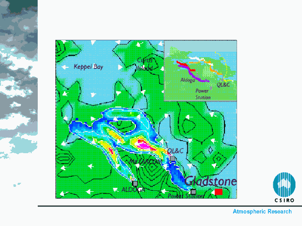
An example of LADM output

• NO2, early morning
  • output data
    • produces pollutant concentration fields at given times (say hourly), use these to study population exposure
    • use specific time and place - direct comparisons with observations (time series, etc.)
    • like Eulerian models (but restricted to fair weather)

• The above plots shows Gladstone example - high concentrations behind hill

Slide 18 of 20

TAPM - CSIRO Atmospheric Research 3-D model (more details at TAPM Web Page)

• Sophisticated 3-D, easy to use and run on a PC
• Appropriate to talk about TAPM even though it’s an Eulerian model, it can do what ‘dispersion’ models do and relatively quickly (it can be run for a year, etc)
• Dispersion modules - Eulerian Grid Module and Lagrangian Particle Module for predicting concentrations very close to the source
• On-line prognostic meteorology module with input from Bureau of Meteorology Limited Area Prediction System data (LAPS data)
• Predicts pollution parameters directly on local, city or inter-regional scales
• Can be run for long time periods
• Gas-phase photochemical reactions based on Generic Reaction Set
• Gaseous- and aqueous-phase chemical reactions for SO2 and fine particles therefore can predict primary and secondary pollutants
• Connected to databases for meteorology, terrain and vegetation, and, therefore, user only needs to input appropriate emissions information, no local meteorology data needed
• Run for periods of a day to a year or more (1997 onwards)- runs relatively quickly on a PC
• Can produce meteorology files for input to regulatory models AUSPLUME, (AUSPUFF), and DISPMOD
• Uses input from Bureau of Meteorology Limited Area Prediction System

Slide 19 of 20

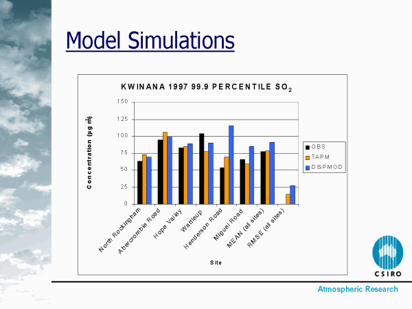
• Kwinana run
  • joint project - CAR and WA DEP
  • WA DEP provided
    • hourly SO2 emission data
    • monitor data
    • DISPMOD run results
  • the above plot shows the 9th highest hourly averaged SO2 ground level concentrations
• TAPM output
  • TAPM can produce output in same form as regulatory models. It can also produce specific time/place output - study population exposure

Slide 20 of 20

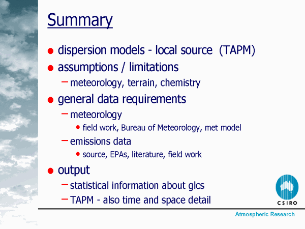
Summary

• Dispersion models
  • modelling a local source or sources with the prime interest in the region close to the source (near source ground level concentrations)
  • TAPM does this as well as regional-scale modelling (TAPM Home Page)

• Assumptions / limitations
  • common assumptions include simple meteorology, simple representation of the effects of terrain (no complex terrain), and no or simple chemical transformations
  • often their underlying assumptions are not valid at larger scales, e.g. sea-breezes, valley flows, recirculation of air (polluted/clean)

• Input data
  • meteorology - simple hourly file surface winds and temperatures, record mixing height, stability class (surface radiation, cloud), (field work, Bureau of Meteorology), more complex meteorology file - meteorological model.
  • emission rates for all pollutants that you want to study, time variation, data about sources eg. height, exit velocity and temperature if buoyant plume - get this info from source, EPAs, literature, field work etc
  • can be difficult

• Models designed to output various quantities that are generally required for cf. with air quality standards
  • average concentrations of pollutants over specified time periods
  • highest ground level concentrations for a pollutant over a region or at certain locations within the region
  • models not used to predict glc info at a specific time and place - average quantities