Research

The air chemistry model

Photochemical transformation mechanisms are used by CSIRO to model the transformation of oxides of nitrogen (NO_x = nitric oxide plus nitrogen dioxide) and volatile organic compounds (VOC) into secondary products such as ozone, hydrogen peroxide, nitric acid and secondary aerosols.

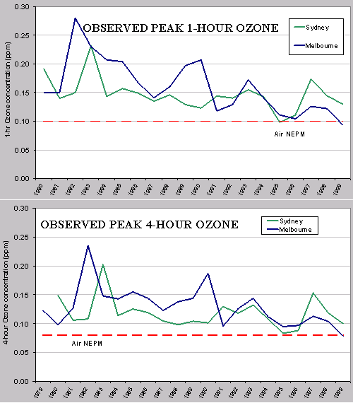
One of the principal secondary pollutants of concern is ozone, which can lead to acute health effects in humans, reduced yields in crops and damage to infrastructures. Health is protected by two National Air Pollution Measures (NEPM; a 1-hour average standard of 0.1° ppm and a 4-hour average standard of 0.08° ppm). Peak ozone concentrations are observed to exceed the NEPM downwind of some large populated regions in Australia (e.g. see for example, 20-year time series for Sydney and Melbourne (Figure 1).

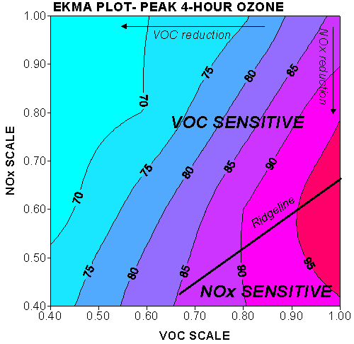
Because the photochemical smog system is strongly non-linear (Figure 2), numerical modelling approaches are generally used to examine the relationship between photochemical smog production and source concentration.

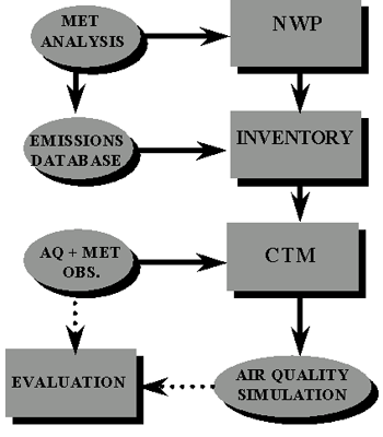
A photochemical air quality modelling system (PAQMS- Figure 3) will typically consist of a numerical weather prediction system, an emissions module and a chemical/transport model. At CSIRO these components are provided by TAPM, a fully integrated weather prediction chemical/transport modelling system, and by the Australian Air Quality Forecasting System (AAQFS), a chemical/transport system which is operated in conjunction with the Bureau of Meteorology Limited Area Prediction System, or with TAPM. 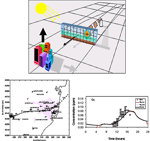CSIRO has also developed a two-dimensional Lagrangian photochemical wall model, which is used for near-field, high-resolution geometries (Figure 4).

The CSIRO PAQMS are principally used in two roles

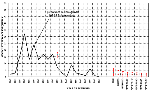
1. As input to strategic policy development. In this role, PAQMS may be used to provide source sensitivity analysis in which the controlling precursor (i.e. whether NO_x or VOC) is determined (Figure 2), and, for the controlling precursor, the most significant source group identified. PAQMS may also be used to look at long-term trends in the peak concentrations of photochemical smog (Figure 5).
2. Provide short-term air quality forecasts to state environment protection authorities for input into their daily smog forecasting schemes. AAQFS is currently used to generate twice-daily forecasts for the Environment Protection Authority of Victoria and for the Environment Protection Authority of NSW.

PAQMS are complex systems whose outputs can often be applied to high-stake policy development. Careful scrutiny of the input and output data streams is an important component of a PAQMS application. CSIRO has developed methodologies for validating major components of a PAQMS. For example, the FAME system is a measurement methodology that has been used with good success to verify fleet average emission estimates for motor vehicles.

Detailed verification for the photochemical transformation mechanism is also available using an indoor environmental smog chamber, recently developed at CSIRO Energy Technology.

Our photochemical air quality modelling systems are continuing to develop, with refinements being made to the meteorological modelling processes, inventory development and validation techniques, and the expansion of the chemical/transport model to include primary and secondary aerosol processes.

Figure 1.

Peak observed 1-hour (top) and 4-hour (bottom) ozone concentrations for a 20-year period spanning 1980-1999 for Melbourne and Sydney.

Figure 2.

Demonstration of non-linearity of the photochemical smog system. The figure shows the (simulated) relationship between peak 4-hour ozone concentration and scaled emission rates of anthropogenic NOx and VOC sources for an Australian airshed. Base-case is represented at the top right-hand corner of the plot and corresponds to NOx and VOC emissions scaled by 1.0 (i.e. un-modified). Cases in which VOC emissions are scaled while NOx emissions are held at base-case totals correspond to moving along the top axis of the plot. Cases in which VOC emissions are held at base-case totals and NOx is reduced correspond to moving down the right-hand axis of the plot. It can be seen that the peak ozone concentrations monotonically decrease as VOC emission rate decreases. On the other hand, ozone first increases and then decreases as the NOx emission rate decreases. Thus the photochemical smog system represented by this plot is a non-linear function of the emission rate of VOC and NOx.

Figure 3.

Schematic diagram of a photochemical air quality modelling system (PAQMS). NWP- the numerical weather prediction system generates vector wind fields and fields of temperature, humidity, radiation and turbulence. The inventory provides data sets of precursor emissions from quantifiable anthropogenic and natural sources. Some emission groups are a function of meteorology, hence the coupling between the NWP and the inventory. CTM- the chemical/transport model converts precursors concentrations into secondary photochemical products. The CTM also models the processes of advection and diffusion. In some fully online models, the predicted gaseous and aerosol trace-species pollutants may feed back into the NWP, impacting on the predictions of radiation and cloud cover.

Figure 4.

Top- schematic diagram of the Lagrangian photochemical wall model. Emissions, diffusion and chemical transformation are modelled in each cell of the wall as it is advected downwind. Bottom left- Trajectory taken by the Lagrangian wall model as it is advected inland over urban Sydney for a photochemical smog event in 1997. Bottom right- observed (error bars) and predicted (solid lines) ozone concentrations for the air parcel trajectory defined in the previous plot.

Figure 5.

Example of trend modelling undertaken using a photochemical smog modelling system for the Port Phillip Control Region (includes Melbourne and Geelong). In this example, the exceedance frequency (days) for the 0.01 ppm National Air Pollution Measure for ozone is modelled (error bars) for a range of 2005 motor vehicle emission scenarios. Also shown (solid line) is the observed exceedance frequency for the period 1980?1999.

[top]

Modified: 9/10/08